I delve into a diverse range of topics, spanning programming languages, machine learning, data engineering tools, and DevOps. Our articles are enriched with practical code examples, ensuring their applicability in real-world scenarios.
Showing posts with label PyTorch. Show all posts
Showing posts with label PyTorch. Show all posts
Tuesday, February 11, 2025
Posts History
Labels:
Airflow,
BERT,
Big Data,
ChatGPT,
Data pipelines,
Deep learning,
Docker,
Genetic Algorithm,
Java,
Kafka,
Machine learning,
Monads,
NoSQL,
Python,
PyTorch,
Reinforcement Learning,
Scala,
Spark,
Streaming
Friday, November 15, 2024
Deep Learning on Mac Laptop with MPS
Target audience: Beginner
Estimated reading time: 5'
Newsletter: Geometric Learning in Python
The latest high-performance Mac laptops are well-suited for experimentation. However, have you been frustrated by your model training running out of memory on an MPS processor?
This article presents a series of techniques and recommendations to effectively manage the memory available on MPS devices in Mac laptops powered by M1, M2, and M3 chips
What you will learn: How to implement and assess different techniques for reducing memory consumption on an MPS device.
Notes:
- Environments: Python 3.12, Matplotlib 3.9, PyTorch 2.4.1
- Source code is available at github.com/patnicolas/geometriclearning/dl/training
- To enhance the readability of the algorithm implementations, we have omitted non-essential code elements like error checking, comments, exceptions, validation of class and method arguments, scoping qualifiers, and import statement.
Metal Performance Shaders (MPS)
The MPS (Metal Performance Shaders) device on macOS enables high-performance GPU acceleration for machine learning tasks, particularly within the PyTorch framework. By leveraging Apple's Metal framework, MPS allows developers to execute computationally intensive operations directly on the GPU [ref 1].
Key Characteristics of the MPS Device:
- Integration with PyTorch: PyTorch allows tensors and models to be allocated and executed on the MPS device. This integration facilitates seamless GPU acceleration for training and inference tasks on macOS.
- Unified Memory Architecture: Apple's unified memory architecture provides the GPU with direct access to the entire memory store.
- Device Compatibility: The MPS backend is compatible with Mac computers equipped with Apple silicon (M1, M2, M3) or AMD GPUs
- Performance Optimization: MPS optimizes compute performance with kernels fine-tuned for the unique characteristics of each Metal GPU family.
Memory optimization techniques
This list of recommendations may not be comprehensive, and some readers might have experimented with other techniques. While a subset of these techniques is implemented and evaluated using PyTorch [ref 2], similar implementations are available in other deep learning frameworks like TensorFlow.
1. Reducing batch size
Batch size directly impacts memory usage, so reducing it is often the most effective way to avoid memory overflow.2. Using mixed precision float values
The MPS backend on macOS doesn’t support
The MPS backend on macOS doesn’t support
torch.cuda.amp.GradScaler, but you can still implement mixed-precision training manually by converting input data to float16 while keeping model weights in float32.3. Checkpointing gradients
Gradient checkpointing (a.k.a. "activation checkpointing") saves memory by storing only a few intermediate activations and recomputing them during backpropagation (
Gradient checkpointing (a.k.a. "activation checkpointing") saves memory by storing only a few intermediate activations and recomputing them during backpropagation (
torch.utils.checkpoint)4. Limiting the number of layers
Use fewer layers or smaller layer sizes to reduce memory requirements (i.e. num filters for CNNs, number of units for fully connected layers)
Use fewer layers or smaller layer sizes to reduce memory requirements (i.e. num filters for CNNs, number of units for fully connected layers)
5. Clearing unused Variables and emptying cacheRemove unused variables withdeland clear cached memory withtorch.mps.empty_cache()to free up memory.This can be helpful in managingmemory between iterations and preventing memory buildup.
6. Using smaller input image resolutions
Resize input images to smaller resolutions to save memory during training.7. Optimizing data Loading with data loaders
Enablepin_memory=Trueto make data transfer to the GPU faster, though youmay need to test if this impacts performance.
8. Accumulating gradients for large effective batch sizesAccumulate gradients over several forward passes and update the modelweights after a specified number of iterations.
9. Reducing memory reserved by the MPS Backend
You can adjust the
You can adjust the
PYTORCH_MPS_HIGH_WATERMARK_RATIO environment variable to control the amount of memory that the MPS backend can use.10. Sampling training data set
Reduce the size of the training set, at least as initial step
11. Monitoring memory consumption
Implementation
Our straightforward implementation uses a class,
ExecConfig, which encapsulates all the recommendations as variables and methods.Setup
We implement 6 of the recommendations described in the previous paragraph, by defining a pair of
- variable enabling the featured recommendation
- method implementing the execution of the recommendation.
class ExecConfig(object):
  def __init__(self,
               empty_cache: bool,
               mix_precision: bool,
               subset_size: int,
               monitor_memory: bool,
               grad_accu_steps: int = 1,
               device_config: AnyStr = None,
               pin_mem: bool = True):
    self.empty_cache = empty_cache
    self.mix_precision = mix_precision
    self.subset_size = subset_size
    self.grad_accu_steps = grad_accu_steps
    self.device_config = device_config
    self.pin_mem = pin_mem
    self.monitor_memory = monitor_memory
# Recommendation 11 def apply_monitor_memory(self) -> None:
# Recommendation 8 def apply_grad_accu_steps(self, idx: int, optimizer: Optimizer) -> None:
    # Recommendation 2
    def apply_mix_precision(self, x: torch.Tensor) -> torch.Tensor:
# Recommendation 5 def apply_empty_cache(self) -> None:
# Recommendation 10def apply_sampling(self,train_dataset: Dataset,test_dataset: Dataset) -> (Dataset, Dataset):# Recommendation 7def apply_optimize_loaders(self, batch_size: int, train_dataset: Dataset, test_dataset: Dataset) -> (DataLoader, DataLoader):
Now let's dive into the implementation of these recommendations.
Recommendations
Monitoring memory consumption [11]
If MPS memory is enabled and the specified device is set to 'mps,' we calculate the total memory available on the MPS device, as well as the memory allocated for training and its usage.
def apply_monitor_memory(self) -> None:if self.monitor_memory and self.device_config == 'mps': allocated_mem = torch.mps.current_allocated_memory() total_mem = torch.mps.driver_allocated_memory() usage = 100.0*allocated_mem/total_mem print(f'\nAllocated MPS: {format(allocated_mem, ",")}' f'\nTotal MPS: {format(total_mem, ",")}' f'\nUsage MPS: {usage:.2f}' )
Accumulating gradients [8]
Gradient computation and subsequent resetting to zero are performed either for each batch (grad_accu_steps = 1) or after every
grad_accu_steps batches.def apply_grad_accu_steps(self, idx: int, optimizer: Optimizer) -> None:
if self.grad_accu_steps == 1 or (idx+1) % self.grad_accu_steps == 0: optimizer.step() optimizer.zero_grad()
Using mixed precision [2]
There are various strategies for incorporating
float16 in the forward and backward passes of the training process. For simplicity, we choose to convert input data from float32 to float16 using the PyTorch half() method.1 2 | def apply_mix_precision(self, x: torch.Tensor) -> torch.Tensor:
return x.half() if self.mix_precision else x
|
Emptying cache [5]
The method torch method, mps.empty_cache() is invoked at the end of each batch, if the recommendation/feature empty_cache is enabled (True).
1
2
3 | def apply_empty_cache(self) -> None:
if self.empty_cache:
torch.mps.empty_cache()
|
Sampling training data [10]
Reducing the size of the training set is a key strategy for minimizing memory consumption. This approach utilizes the
Subset class from the PyTorch library. A key challenge is re-indexing the training data points by setting indices=range(subset_size).def apply_sampling(self,
train_dataset: Dataset,
test_dataset: Dataset) -> (Dataset, Dataset):
if self.subset_size > 0:
from torch.utils.data import Subset
# Rescale the size of training and test data
test_sub_size = int(float(self.subset_size * len(test_dataset)) / len(train_dataset))
train_sub_size = self.subset_size - test_subset_size
      # Re-index the subset of training and test data set
      train_dataset = Subset(train_dataset, indices=range(train_sub_size))
      test_dataset = Subset(test_dataset, indices=range(test_sub_size))
return train_dataset, test_dataset
Optimizing data Loading [7]
The final recommendation we assess involves pinning memory to optimize the transfer of training data points from the CPU to the GPU.
def apply_optimize_loaders(self,
                      batch_size: int,
                      train_dataset: Dataset,
                      test_dataset: Dataset) -> (DataLoader, DataLoader):
   train_loader = DataLoader(
            dataset=train_dataset,
            batch_size=batch_size,
            pin_memory=self.pin_mem,  # Recommendation #7
            shuffle=True)
   test_loader = DataLoader(
            dataset=test_dataset,
            batch_size=batch_size,
            pin_memory=self.pin_mem,
            shuffle=False)
return train_loader, test_loader
Evaluation
MNIST is a database of handwritten digits with of 60,000 training examples and 10,000 examples [ref 3]
Caltech101 is a well-known dataset of 9146 images from 102 categories from airplanes, animal to furniture [ref 4]
The next step involves incorporating the six recommendations into the processes of loading and training the MNIST and Caltech101 datasets. To achieve this, we encapsulate the data loading and model training within a class called NeuraNet. For simplicity, the implementation is streamlined to include only the essential attributes required for training and validating the model:
- model: A convolutional neural network.
- metrics: A dictionary containing metrics such as precision and recall.
- exec_config: The training execution configuration, as defined in the previous section.
class NeuralNet(object):
    def __init__(self,
                 model: nn.Module,
                 metrics: Dict[AnyStr, Metric],
exec_config: ExecConfig) -> None:self.model = model.to(self.target_device) self.exec_config = exec_config self.metrics = metrics
We apply the sampling of training data (subset) to the data loaded from local files. Then
we enabled memory pinning to optimize the data loaders.
def load_dataset(self, train_dataset : Dataset, test_dataset: Dataset) -> (DataLoader, DataLoader):
# Sample training data - Recommendation #10 train_dataset, test_dataset = exec_config.apply_sampling( train_dataset, test_dataset ) # Optimize data loaders - Recommendation #7 train_loader, test_loader = exec_config.apply_optimizing_loaders( train_dataset, test_dataset )
return train_loader, test_loaderThe following code snippet illustrates the standard training approach, which involves training on a subset or the entire dataset, followed by validation and the calculation of key performance metrics. Non essential ancillary and debugging statement are omitted.
Additionally, memory usage on the MPS device (recommendation 11) is measured at the end of each epoch.
def train(self,
              train_loader: DataLoader,
              test_loader: DataLoader) -> None:

    torch.manual_seed(42)
    initialize_weight(list(self.model.modules()))

        # Train and evaluation process
    for epoch in tqdm(range(self.epochs)):
       # Training
       train_loss = self.__train(epoch, train_loader)
       # Evaluation and computation of metrics (F1, ...)
       eval_metrics = self.__eval(epoch, test_loader)
      # Initialize monitoring of memory on mps device
       self.exec_config.apply_monitor_memory()  # Recommendation11
The private method
__train performs training on the dataset for each epoch. For every batch, the cache is cleared, and gradient values are accumulated.def __train(self, epoch: int, train_loader: DataLoader) -> float:
total_loss = 0.0
    # Initialize the gradient for the optimizer
    loss_function = self.loss_function
    optimizer = self.optimizer(self.model)
    self.model.to(torch_device)

    for idx, (features, labels) in enumerate(train_loader):
        model.train()

        features = features.to(torch_device)
        labels = labels.to(torch_device)
        predicted = model(features)  # Call forward - prediction
        raw_loss = loss_function(predicted, labels)

        # Set back propagation
        raw_loss.backward(retain_graph=True)
        total_loss += raw_loss.data
# MPS memory management --------------------- # 3 Cache management self.exec_config.apply_empty_cache() # 4 Aggregation grad steps
self.exec_config.apply_grad_accu_steps(idx, optimizer)
return total_loss / len(train_loader)
We conduct a binary test [ON/OFF] for each recommendation and track its impact on memory availability for the MPS device:
- Using 20% of the dataset vs. the entire dataset
- Enabling vs. disabling memory pinning
- Using mixed precision (
float16) for training data vs. full precision - Enabling vs. disabling cache clearing between batches
- Accumulating gradients over multiple batches vs. single-batch accumulation
-------------
Patrick Nicolas has over 25 years of experience in software and data engineering, architecture design and end-to-end deployment and support with extensive knowledge in machine learning.
He has been director of data engineering at Aideo Technologies since 2017 and he is the author of "Scala for Machine Learning", Packt Publishing ISBN 978-1-78712-238-3 and Geometric Learning in Python Newsletter on LinkedIn.
Appendix
Architecture of the convolutional neural network used to evaluate the recommended memory reduction policies.
- Conv2d(3, 64, kernel_size=(3, 3), stride=(1, 1), bias=False)
- BatchNorm2d(64, eps=1e-05, momentum=0.1, affine=True, track_running_stats=Tru e)
- ReLU()
- MaxPool2d(kernel_size=2, stride=1, padding=0, dilation=1, ceil_mode=False)
- Conv2d(64, 128, kernel_size=(3, 3), stride=(1, 1), bias=False)
- BatchNorm2d(128, eps=1e-05, momentum=0.1, affine=True, track_running_stats=True)
- MaxPool2d(kernel_size=2, stride=1, padding=0, dilation=1, ceil_mode=False)
- Conv2d(128, 256, kernel_size=(3, 3), stride=(1, 1), bias=False)
- BatchNorm2d(256,eps=1e-05,momentum=0.1,affine=True, track_running_stats=True)
- MaxPool2d(kernel_size=2, stride=1, padding=0, dilation=1, ceil_mode=False)
- Conv2d(256, 512, kernel_size=(3, 3), stride=(1, 1), bias=False)
- BatchNorm2d(512, eps=1e-05, momentum=0.1, affine=True, track_running_stats=True)
- MaxPool2d(kernel_size=2, stride=1, padding=0, dilation=1, ceil_mode=False)
- Flatten(start_dim=1, end_dim=-1)
- Linear(in_features=3612672, out_features=512, bias=False)
- Linear(in_features=512, out_features=101, bias=False)
- Softmax(dim=1)
Thursday, October 31, 2024
Impact of Linear Activation on Convolution Networks
Target audience: Beginner
Estimated reading time: 5'
Newsletter: Geometric Learning in Python
Have you ever wondered how choosing an activation function can influence the performance of a convolutional neural network?
This article demonstrates the effect of different linear units on the performance and test loss of the classification of MNIST data.
What you will learn: How various activation functions impact the performance of a convolutional neural network.
Notes:
- Environments: Python 3.11, Matplotlib 3.9, PyTorch 2.4.1
- Source code is available at github.com/patnicolas/geometriclearning/dl/model/vision
- To enhance the readability of the algorithm implementations, we have omitted non-essential code elements like error checking, comments, exceptions, validation of class and method arguments, scoping qualifiers, and import statement.
Introduction
The choice of activation function(s) for a neural network depends on the type of input data (such as images, text, signals, sound, video, etc.). Many machine learning practitioners often default to using the Rectified Linear Unit (ReLU) for convenience. However, exploring alternative activation functions can be beneficial, as it provides insights into their unique properties and their impact on the training quality for a specific model.
The MNIST database [ref 1], which stands for Modified National Institute of Standards and Technology database, is a large collection of handwritten digit images commonly used for training various image processing systems. It is widely employed for training and testing purposes in the field of machine learning.
The MNIST database contains 60,000 training images and 10,000 testing images.
The classification problem consists of identifying any of the 10 handwritten digits.
Our model
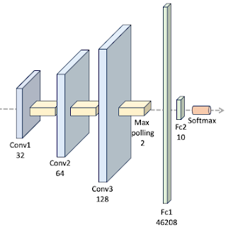
There are various proposed architectures for the training and testing against MNIST data set [ref 2]. We select a 3 layer convolutional neural network followed by two feed forward networks as illustrated below:
We utilize the standard network layer configuration for processing the MNIST dataset.
The ConvNet class is implemented as a PyTorch module [ref 3], handling the model's specification, training, and evaluation. Since the activation function is the sole parameter under evaluation in this study, it is provided as a callable function argument in the constructor.
Each digit is represented as a label in this classification model.
class ConvNet(nn.Module):
    num_classes = 10

def __init__( self, activation: Callable[[torch.Tensor], torch.Tensor]) -> None:
super(ConvNet, self).__init__()
         # Convolutional layers
        self.conv1 = nn.Conv2d(in_channels=1,
out_channels=32, kernel_size=3, stride=1)
self.bn1 = nn.BatchNorm2d(32) self.conv2 = nn.Conv2d(in_channels=32, out_channels=64, kernel_size=3, stride=1)
self.bn2 = nn.BatchNorm2d(64) self.conv3 = nn.Conv2d(in_channels=64, out_channels=128, kernel_size=3, stride=1) self.bn3 = nn.BatchNorm2d(128)
# Drop out shared by all layers self.dropout = nn.Dropout(0.15)
        # Fully connected layers
        in_fc = 46208
        self.fc1 = nn.Linear(in_features=in_fc,
                                       out_features=128)
        self.fc2 = nn.Linear(in_features=128,
out_features=ConvNet.num_classes)
         # Activation function shared by all layers
        self.activation = activation
.
For the sake of simplicity, the various layers of the model share the same dropout (regularization) factor and activation function. The forward method implements the flow of data through the 3 convolutional blocks (convolution, batch normalization, max pooling, activation and drop out.
def forward(self, x: torch.Tensor) -> torch.Tensor:
    # First conv block
    x = self.conv1(x)
    x = self.bn1(x)
    x = F.max_pool2d(x, kernel_size=2)
    x = self.activation(x)
    x = self.dropout(x)

    # Second conv block
    x = self.conv2(x)
    x = self.bn2(x)
    x = F.max_pool2d(x, kernel_size=2)
    x = self.activation(x)
    x = self.dropout(x)

    # Third conv block
    x = self.conv3(x)
    x = self.bn3(x)
    x = F.max_pool2d(x, kernel_size=2)
    x = self.activation(x)
    x = self.dropout(x)

    x = torch.flatten(x, 1)
    # First FFNN block
    x = self.fc1(x)
    x = self.activation (x)

    # Last layer with soft max for output [0, 1]
    x = self.fc2(x)
    return F.log_softmax(x, dim=1)
Training and evaluation are performed with the following hyper-parameters:
- Optimizer: Adam
Learning rate: 0.006
Momentum: 0.89
- Batch size: 32
- Num of epochs: 10
- train to eval ratio: 0.92
- Normal weight initialization: Disabled
- Loss function: Cross entropy
Learning rate: 0.006
Momentum: 0.89
- Batch size: 32
- Num of epochs: 10
- train to eval ratio: 0.92
- Normal weight initialization: Disabled
- Loss function: Cross entropy
The reference implementation of the training and evaluation of the convolutional network in PyTorch is shown in the Appendix.
Evaluation
We compare the following four activation functions:
- Rectified linear unit
- Leaky rectified linear unit
- Exponential linear unit
- Gaussian error linear unit
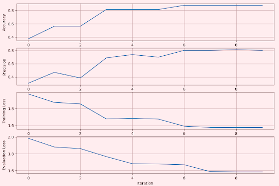
We record and plot the accuracy, precision, training and evaluation loss for the models associated with these activation functions.
Rectified Linear Unit
The Rectified Linear Unit (ReLU), is a widely used activation function in neural networks. It introduces non-linearity into the model, enabling it to learn complex patterns.
Fig. 2 Metrics for Convolutional Network using Rectified Linear Unit - MNIST
Leaky Rectified Linear Unit
Leaky ReLU is a variant of the Rectified Linear Unit (ReLU) activation function used. It address the "dying ReLU" problem, where neurons can stop learning if they consistently output zero. Leaky ReLU introduces a small, non-zero gradient for negative input values, allowing neurons to remain active even when receiving negative inputs.
We use a negative slope of 0.002
Fig. 3 Metrics for Convolutional Network using Leaky Rectifier Linear Unit - MNIST
Exponential Linear Unit
Fig. 4 Metrics for Convolutional Network using Exponential Linear Unit - MNIST
Gaussian Error Linear Unit
The Gaussian Error Linear Unit (GELU) is an activation function popular in transformer architectures (such as BERT and other NLP models)
Fig. 5 Metrics for Convolutional Network using Gaussian Error Linear Unit - MNIST
Analysis
Let's compare the impact of then 4 activation functions on F1 score and evaluation loss.
Fig 6 Impact of selection of activation functions on F1 score for MNIST dataset
The model using exponential linear unit is the only one which F1 score converges quickly to 1.0. All other models have a F1 score of 0.84-0.85. As expected the model ReLU is the slowest to converge.
Fig 7 Impact of selection of activation functions on evaluation loss for MNIST dataset
The loss function profile for the test dataset of each model reflects the previous F1 score plot: the exponential linear unit shows the lowest loss, while the other three models converge toward a similar loss value. ReLU exhibits the slowest convergence profile.
Subscribe to:
Posts (Atom)


