Thursday, December 7, 2017

Category Theory in Scala 2.x

Target audience: Advanced
Estimated reading time: 6'

"Mathematics is security. Certainty. Truth. Beauty. Insight. Structure. Architecture. Whether it is differential topology, or functional analysis, or homological algebra, it is all one thing. ..."  Paul Halmos


Table of contents
Notes
  • This post requires a solid knowledge of functional programming as well understanding of differential geometry.
  • Implementation relies on Scala 2.12.10

Overview

Scala is a premier language that seamlessly integrates functional programming and object-oriented paradigms, supporting various advanced concepts including higher-kind types, functors, and monads. This article demonstrates Scala's ability to utilize covariant and contravariant functors for tensor analysis, particularly in the context of vector field applications.

Many Scala developers are familiar with key functional programming principles such as monads, functors, and applicatives. However, these concepts extend beyond Scala and functional programming in general. They originate from areas in mathematics like topology and algebraic topology. In fields such as differential geometry or differential topology, tensors, which utilize covariant and contravariant functors, are extensively employed.

Category theory

Introduction

Category theory is a branch of mathematics that deals with abstract structures and relationships between them. It's a high-level, formal language that's used to unify concepts across various fields of mathematics [ref 1]. Here's a breakdown of its fundamental aspects:
  • Categories: At the heart of category theory are categories. A category consists of objects and morphisms (also called arrows or maps) between these objects. Objects can be anything (sets, spaces, groups, etc.), and morphisms are ways of transforming one object into another. Importantly, these transformations must be able to be composed together, and this composition must be associative. Additionally, for each object, there is an identity morphism that acts neutrally in composition.
  • Morphisms: These are critical in category theory. A morphism represents a relationship or a function between two objects. It's not just a function in the traditional sense; it's a more generalized concept.
  • Functors: These are mappings between categories. A functor respects the structure of categories; it maps objects to objects, morphisms to morphisms, and preserves the composition and identity of morphisms.
  • Natural Transformations: These provide a way to transform one functor into another while respecting their action on objects and morphisms.
  • Universal Properties: These are properties that define an object in terms of its relationships with other objects, typically describing the 'most efficient' solution to a particular problem.
  • Limits and Colimits: These are concepts that generalize constructions like products, coproducts, intersections, and unions.
Category theory is known for its level of abstraction, making it a powerful tool in unifying concepts across different mathematical disciplines. It has found applications in fields such as algebra, topology, and computer science, particularly in the study of functional programming languages. By providing a high-level language for describing and analyzing mathematical structures, category theory helps reveal deep connections between seemingly disparate areas of mathematics.

Covariant functors

A covariant functor F from the category of topological spaces T to some algebraic category C is a function which assigns to each space X an object F(X) in C and to each continuous map f: X → Y a homomorphism F(f): F(X) → F(Y) with \[F(f\circ g)=F(f)\circ F(g)\begin{matrix} & F(id_{X})=id_{Y} \end{matrix}\]

I assume the reader has basic understanding of Functors [ref 2]. Here is short overview:
category C is composed of object x and morphism f defined as
\[C= \{ {x_{i}, f \in C | f: x_{i} \mapsto x_{j}} \}\] A functor F is a map between two categories C and D that preserves the mapping.
\[x\in C \Rightarrow F(x)\in D \\ x, y\in C \,\,\, F: x \mapsto y => F(x)\mapsto F(y)\] 
Let's look at the definition of a functor in Scala with the "preserving" mapping method, map

trait Functor[M[_]] {
     def map[U, V](m: M[U])(f: U => V): M[V]
}

Let's define the functor for a vector (or tensor) field. A vector field is defined as a sequence or list of fields (i.e. values or function values).
type VField[U] = List[U]

trait VField_Ftor extends Functor[VField] {
      override def map[U, V](vu: VField[U])(f: U => V): VField[V] = vu.map(f) 
}

This particular implementation relies on the fact that List is a category with its own functor. The next step is to define the implicit class conversion VField[U] => Functor[VField[U]] so the map method is automatically invoked for each VField instance.
implicit class vField2Functor[U](vu: VField[U]) extends VField_Ftor {  
    
  final def map[V](f: U => V): VField[V] = super.map(vu)(f) 
}

By default Covariant Functors (which preserve mapping) are known simply as Functors. Let's look at the case of Covector fields.

Contravariant functors

A contravariant functor G is similar to covariant functors. G(f) is a homomorphism from G(Y) to G(X) with \[G(f\circ g)=G(g)\circ G(f)\begin{matrix} & G(id_{X})=id_{Y} \end{matrix}\] Contravariant functor is a map between two categories that reverses the mapping of morphisms.
\[x, y\in C \,\,\, G: x \mapsto y => G(y)\mapsto G(x)\]
trait CoFunctor[M[_]] {
     
   def map[U, V](m: M[U])(f: V => U): M[V]
}

The map method of the Cofunctor implements the relation M[V->U] => M[U]->M[V]
Let's implement a co-vector field using a contravariant functor. The definition  describes a linear map between a vector V over a field X to the scalar product  V*: V => T.
A morphism on the category V* consists of a morphism of V => T or V => _ where is a vector field and T or _ is a scalar function value.
type CoField[V, T] = Function1[V, T] 

The co-vector field type, CoField is parameterized on the vector field type V which is a input or function parameter. Therefore the functor has to be contravariant.

The higher kind type M[_] takes a single type as parameter (i.e. M[V]) but a co-vector field requires two types:
  • V: Vector field
  • T: The scalar function is that the result of the inner product <.>
Fortunately the contravariant functor CoField_Ftor associated with the co-vector needs to be parameterized only with the vector field V. The solution is to pre-defined (or 'fix') the scalar type T using a higher kind projector for the type L[V] => CoField[V, T]     T => ({type L[X] = CoField[X,T]})#L

trait CoField_Ftor[T]  extends CoFunctor[({type L[X] = CoField[X,T]})#L ] {

  override def map[U,V](vu: CoField[U,T])(f: V => U): CoField[V,T] =  
    (v: V) => vu(f(v))
}

As you can see the morphism over the type V on the category CoField is defined as f: V => U instead of f: U => V. A kind parameterized on the return type (Function1) would require the 'default' (covariant) functor. Once again, we define an implicit class to convert a co-vector field, of type CoField to its functor, CoField2Ftor
implicit class CoField2Ftor [U,T](vu: CoField[U,T])  extends CoField_Ftor {
 
  final def map[V](f: V => U): CoField[V,T] = super.map(vu)(f) 
}

Monads

A monad is a concept from category theory, a branch of mathematics, which has become particularly important in functional programming. It's a way to represent computations as a series of actions in a specific context, providing a framework for handling side effects, manipulating data, and structuring programs. 
A monad is a type of functor, a structure that applies a function to values wrapped in a context. 
In functional programming, monads offer a way to deal with side effects (like state, IO,) while keeping the pure functional nature of the code. A monad can be then defined by its 3 methods: unit, map & flatMap [ref 3].

trait Monad[M[_]] {
  def unit[T](t: T): M[T]
  def map[T, U](m: M[T])(f: T => U): M[U]
  def flatMap[T, U](m: M[T])(f: T => M[U]): M[U]
}

Example for List:
  • unit(str: String) = List[String](str))
  • map(f: (str: String) => str.toUpperCase) = List[String](str.toUpperCase))
  • flatMap (f: (str: String) => List[String](str.toUpperCase))  =  List[String](str.toUpperCase))

Application to differential geometry

Category theory is applicable to differential geometry and tensor analysis on manifolds [ref 4]

Vector fields

Let's consider a 3 dimension Euclidean space with basis vector {ei} and a vector field V (f1, f2, f3) [Note: we follow Einstein tensor indices convention]

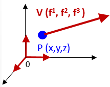
The vector field at the point P(x,y,z) as the tuple (f1(x,y,z), f2(x,y,z), f3(x,y,z)).
The vector over a field of k dimension field can be formally. mathematically defined as 
\[f: \boldsymbol{x} \,\, \epsilon \,\,\, \mathbb{R}^{k} \mapsto \mathbb{R} \\ f(\mathbf{x})=\sum_{i=1}^{n}{f^{i}}(\mathbf{x}).\mathbf{e}^{i}\] Example: \[f(x,y,z) = (2x+z^{3})\boldsymbol{\mathbf{\overrightarrow{i}}} + (xy+e^{-y}-z^{2})\boldsymbol{\mathbf{\overrightarrow{j}}} + \frac{x^{3}}{y}\boldsymbol{\mathbf{\overrightarrow{k}}}\] Now, let's consider the  same vector V with a second reference (origin O' and basis vector e'i).

\[f(\mathbf{x})=\sum_{i=1}^{n}{f'_{i}}(\mathbf{x}).\mathbf{e'}_{i}\]
The transformation matrix Sij convert the coordinates value functions fi and f'i. The tuple f =(fi) or more accurately defined as (fi) is the co-vector field for the vector field V
\[S_{ij}: \begin{Vmatrix} f^{1} \\ f^{2} \\ f^{3} \end{Vmatrix} \mapsto \begin{Vmatrix} f'^{1} \\ f'^{2} \\ f'^{3} \end{Vmatrix}\]
The scalar product of the co-vector f' and vector v(f) defined as is defined as
\[< f',v> = \sum f'_{i}.f^{i}\]
Given the scalar product we can define the co-vector field f' as a linear map
\[\alpha (v) = < f',v> (1) \] 


Functors for vector fields

Now we can apply functors to operations on vector fields  [ref 5].

Let's consider a field of function values FuncD of two dimension: v(x,y) = f1(x,y).i + f2(x,y).j. The Vector field VFieldD is defined as a list of two function values.
type DVector = Array[Double]
type FuncD = Function1[DVector, Double]
type VFieldD = VField[FuncD] 

The vector is computed by assigning a vector field to a specific point (P(1.5, 2.0). The functor is applied to the vector field, vField to generate a new vector field vField2
val f1: FuncD = new FuncD((x: DVector) => x(0)*x(1))
val f2: FuncD = new FuncD((x: DVector) => -2.0*x(1)*x(1))
  
val vField: VFieldD = List[FuncD](f1, f2)
val value: DVector = Array[Double](1.5, 2.0)  
val vField2: VFieldD = vfield.map( _*(4.0))


A co-vector field, coField is computed as the sum of the fields (function values) (lines 1, 2). Next, we compute the product of co-vector field and vector field (scalar field product) (line 3). We simply apply the co-vector Cofield (linear map) to the vector field. Once defined, the morphism _morphism is used to generate a new co-vector field coField2 through the contravariant function CoField2Functor.map (line 6).

Finally, a newProduct is generated by composing the original covariant field coField and the linear map coField2 (line 7).

1
2
3
4
5
6
7
val coField: CoField[VFieldD, FuncD] =  (vf: VFieldD) => vf(0) + vf(1)
val contraFtor: CoField2Functor[VFieldD, FuncD] = coField
val product = coField(vField)
val _morphism: VFieldD => VFieldD =  (vf: VFieldD) => vf.map( _*(3.0))

val coField2 = contraFtor.map( _morphism )
val newProduct: FuncD = coField2(coField)

Note: This section on the application of functors to vector fields can be extended to tensor fields and smooth manifolds.

Higher kinds in Scala 3

The implementation of functors in Scala 2 relies on the type system been based on class types first (including traits and object classes), along with type projections of the form T#X. Path-dependent types were described as a combination of singleton types and type projections. 
     ({type R[A+] = Either[Int, A]})#R
     ({type L[B] = Either[B, Int]})#L
Scala 3 modifies the implementation of higher kind projection. It uses the underscore, _, symbol for placeholders in type lambdas [ref 6]. The new, simplified formalism is:
     Either[Int, +_]
     Either[_, Int]
The new formalism can be used with existing code Scala 2 through a migration library [ref 7].


Thank you for reading this article. For more information ...

References

[4] Tensor Analysis on Manifolds- Chap 3 Vector Analysis on Manifolds- R. Bishop, S. Goldberg - Dover publication 1980 
[5Differential Geometric Structures/ Operations on Vector Bundles p20-22 -  W. Poor - Dover publications 2007


---------------------------
Patrick Nicolas has over 25 years of experience in software and data engineering, architecture design and end-to-end deployment and support with extensive knowledge in machine learning. 
He has been director of data engineering at Aideo Technologies since 2017 and he is the author of "Scala for Machine Learning" Packt Publishing ISBN 978-1-78712-238-3

Friday, October 27, 2017

Implement Reinforcement Learning in Scala

Target audience: Advanced
Estimated reading time: 8'

Ever pondered how robots, self-operating systems, or software-based game players acquire knowledge? 
The secret is nestled within an AI branch called reinforcement learning. In this piece, we delve into a widely recognized reinforcement learning technique - Q-learning, and illustrate its implementation in Scala.

What you will learn: Implementation of Q-Learning in Scala

Notes:
  • EnvironmentsScala: 2.12.4, Java JDK 11
  • This article assumes that the reader is familiar with machine learning and computer programming.

Overview

Numerous techniques exist within the field of reinforcement learning. A widely adopted approach involves exploring the value function space through the temporal difference method. Despite their diversity, all reinforcement learning methods converge on a common goal: to solve the challenge of identifying the best sequence of decision-making tasks [ref 1]. In these tasks, an agent engages with a dynamic system, choosing actions that influence state transitions, all with the aim of optimizing a specified reward function.

Basic components of reinforcement learning

At any given step i, the agent selects an action a(i) on the current state s(i). The dynamic system responds by rewarding the agent for its optimal selection of the next state:\[s_{i+1}=V(s_{i})\]
The learning agent infers the policy that maps the set of states {s} to the set of available actions {a}, using a value function  \[V(s_{i})\] The policy is defined at \[\pi :\,\{s_{i}\} \mapsto \{a_{i}\} \left \{ s_{i}|s_{i+1}=V(s_{i}) \right \}\] For example, a robot navigating through a maze makes its next move based on its present location and past actions. It's impractical to instruct the robot on every possible move for each location within the maze, rendering supervised learning techniques insufficient for this task.

Temporal difference

The most common approach of learning a value function V is to use the Temporal Difference method (TD). The method uses observations of prediction differences from consecutive states, s(i) & s(i+1). If we note r the reward for selection an action from state s(i) to s(i+1) and n the learning rate, then the value V is updated as \[V(s_{i})\leftarrow V(s_{i})+\eta .(V(s_{i+1}) -V(s_{i}) + r_{i})\]
Therefore the goal of the temporal difference method is to learn the value function for the optimal policy. The Q 'action-value' function represents the expected value of action a on a state s and defined as \[Q(s_{i},a_{i}) = r(s_{i}) + V(s_{i})\] where r is the reward value for the state.


On-policy vs. Off-policy

The Temporal Difference method calculates an estimated final reward for each state. This method comes in two variations: On-Policy and Off-Policy:
  • The On-Policy approach learns the value of the policy it employs for decision-making. Its value function is based on the outcomes of actions taken under the same policy, but it incorporates historical data.
  • The Off-Policy approach, on the other hand, learns from a variety of potential policies. 
As such, it bases its estimates on actions that have yet to be taken.
A widely used formula in the Temporal Difference approach is the Q-learning formula [ref 2]. This introduces a discount rate to lessen the influence of initial states on policy optimization. It operates without needing a model of the environment. In the action-value method, the selection of the next state involves choosing the action with the highest reward, known as exploitation. In contrast, the exploration approach emphasizes maximizing the total expected reward.
The update equation for the Q-Learning is \[Q(s_{i},a_{i}) \leftarrow Q(s_{i},a_{i}) + \eta .(r_{i+1} +\alpha .max_{a_{i+1}}Q(s_{i+1},a_{i+1}) - Q(s_{i},a_{i}))\]
Q(s,a)expected value action a on state s
eta: learning rate
alpha: discount rate 
One of the most commonly used On-Policy method is Sarsa which does not necessarily select the action that offer the most value.The update equation is defined as\[Q(s_{i},a_{i}) \leftarrow Q(s_{i},a_{i}) + \eta .(r_{i+1} +\alpha .Q(s_{i+1},a_{i+1}) - Q(s_{i},a_{i}))\]

Q-Learning

States & actions

Functional languages are particularly suitable for iterative computation. We use Scala for the implementation of the temporal difference algorithm [ref 3]. We allow the user to specify any variant of the learning formula, using local functions or closures.

Firstly, we have to define a state class, QLState (line 1) that contains a list of actions of type QLAction (line 3) that can be executed from this state. The only purpose of this class is to connect a list of action to a source state. The parameterized class argument property (line 4) is used to "attach" some extra characteristics to this state.

1
2
3
4
5
6
7
8
class QLState[T](
   val id: Int, 
   val actions: List[QLAction[T]] = List.empty, 
    property: T) {
    
  @inline
  def isGoal: Boolean = !actions.isEmpty
}

As described in the introduction, an action of class QLAction has a source state from and a destination state to(state which is reached following the action). A state except the goal state, has multiple actions but an action has only one destination or resulting state.

 case class QLAction[T](from: Int, to: Int) 


The state and action can be processed, created, and overseen using a directed graph or a search domain known as QLSpace. This search domain encompasses all potential states accessible to the agent.

Multiple states from this pool can be designated as objectives, and the algorithm allows the agent to pursue more than one goal state, not just a singular one. The procedure concludes when any of the selected goal states is attained, following an 'OR' logic approach. However, the algorithm does not facilitate the achievement of combined goals, as in an 'AND' logic framework.

Illustration of action-space in reinforcement learning

Let's implement the basic components of the search space QLSpace. The class list all available states (line 2) and one or more final or goal states goalIds (line 3). Although you would expect that the search space contains a single final state (goal) with the highest possible reward, it is not uncommon to have online training using more than one goal states.

 1
 2
 3
 4
 5
 6
 7
 8
 9
10
11
12
13
14
15
16
17
18
19
20
21
22
class QLSpace[T](
   states: Array[QLState[T]], 
   goalIds: Array[Int]) {

    // Indexed map of states 
  val statesMap: immutable.Map[Int, QLState[T]] = 
        states.map(st => (st.id, st)).toMap
    // List set of one or more goals  
  val goalStates = new immutable.HashSet[Int]() ++ goalIds
 
    // Compute the maximum Q value for a given state and policy
  def maxQ(st: QLState[T], policy: QLPolicy[T]): Double = { 
     val best = states.filter( _ != st).maxBy(s => policy.EQ(s.id, s.id))
     policy.EQ(st.id, best.id)
  }
 
    // Retrieves the list of states destination of state, st
  def nextStates(st: QLState[T]): List[QLState[T]] =
     st.actions.map(ac => statesMap.get(ac.to).get)
 
  def init(r: Random): QLState[T] =  states(r.nextInt(states.size-1))
}

A hash map statesMap maintains a dictionary of all the possible states with the state id as unique key (lines 6, 7). The class QLSpace has three important methods: 
  • init initializes the search with a random state for each training epoch (lines 22, 23)
  • nextStates returns the list of destination states associated to the state st (lines 19, 20)
  • maxQ return the maximum Q-value for this state st given the current policy (lines 12-15). The method filters out itself from the search from the next best action. It then computes the maximum reward or Q(state, action) value according to the given policy.
The next step is to define a policy.

Learning policy

A policy is defined by three components:
  • A reward collected after transitioning from one state to another state (line 2). The reward is provided by the user.
  • A Q(State, Action) value associated to a transition state and an action (line 4).
  • A probability (with default values of 1.0) that defines the obstacles or penalties to migrate from one state to another (line 3).
The estimate combines the Q-value (incentive to move to the best next step) and probability (hindrance to move to any particular state) (line 7).

1
2
3
4
5
6
7
8
class QLData {
   var reward: Double = 1.0
   var probability: Double = 1.0
   var value: Double = 0.0) {
  
   @inline
   final def estimate: Double = value*probability
}

The policy of type QLPolicy is a container for the state transition attributes such as a reward, a probability and a value.

 1
 2
 3
 4
 5
 6
 7
 8
 9
10
11
12
13
14
15
16
17
18
19
class QLPolicy[T](numStates: Int, input: Array[QLInput]) {
   val qlData = {
      val data = Array.tabulate(numStates)(
         _ => Array.fill(numStates)(new QLData)
      )

      input.foreach(
        in => {  
           data(in.from)(in.to).reward = in.reward
           data(in.from)(in.to).probability = in.prob
        }
      )
      data
   }
  
   def setQ(from: Int, to: Int, value: Double): Unit =
       qlData(from)(to).value = value
 
   def Q(from: Int, to: Int): Double = qlData(from)(to).value
}

The constructor for QLPolicy takes two arguments:
  • Total number of states numStates used in the search (line 1)
  • Sequence of input of type QLInput to the policy
The constructor creates a numStates x numStates matrix of transition of type QLData (lines 3 - 12), from the input. 
The type QLInput wraps the input data (index of the input state from, index of the output state to, reward and probability associated to the state transition) into a single convenient class.

case class QLInput(
   from: Int,  
   to: Int, 
   reward: Double = 1.0, 
   prob: Double = 1.0)


Model training

The initial phase involves establishing a model for the reinforcement learning. During training, a model, known as QLModel, is constructed and consists of two key components:
  • 'bestPolicy', which delineates the transitions from any starting state to a target state.
  • 'coverage', which indicates the proportion of training cycles that successfully reach the goal state.
class QLModel[T](val bestPolicy: QLPolicy[T], val coverage: Double) 

The QLearning class takes 3 arguments:
  • A set of configuration parameters config.
  • The search/states space qlSpace.
  • The initial policy associated with the states (reward and probabilities) qlPolicy.
 1
 2
 3
 4
 5
 6
 7
 8
 9
10
11
12
13
14
15
16
17
18
19
class QLearning[T](
   config: QLConfig, 
   qlSpace: QLSpace[T], 
   qlPolicy: QLPolicy[T]) 

    //model in Q-learning algorithm
   val model: Option[QLModel[T]] = train.toOption
    
    // Generate a model through multi-epoch training
   def train: Try[Option[QLModel[T]]] {}
   private def train(r: Random): Boolean {}

     // Predict a state as a destination of this current 
     // state, given a model
   def predict : PartialFunction[QLState[T], QLState[T]] {}

     // Select next state and action index
   def nextState(st: (QLState[T], Int)): (QLState[T], Int) {} 
}

The model of type QLModel (line 7) is created as optional by the method train (line 10). Its value is None if training failed.

The training method train consists of executing config.numEpisodes cycle or episode of a sequence of state transition (line 5). The random generator r is used in the initialization of the search space.

 1
 2
 3
 4
 5
 6
 7
 8
 9
10
11
12
13
def train: Option[QLModel[T]] = {
   val r = new Random(System.currentTimeMillis)

   Try {
      val completions = Range(0, config.numEpisodes).filter(train(r) )

      val coverage = completions.toSize.toDouble/config.numEpisodes
      if(coverage > config.minCoverage) 
          new QLModel[T](qlPolicy, coverage)
      else 
          QLModel.empty[T]
    }.toOption
}

The training process exits with the model if the minimum minCoverage (number of episodes for which the goal state is reached) is met (line 8).

The method train(r: scala.util.Random) uses a tail recursion to transition from the initial random state to one of the goal state. The tail recursion is implemented by the search method (line 4). The method implements the recursive temporal difference formula (lines 14-18). 
The state for which the action generates the highest reward R given a policy qlPolicy (line 10) is computed for each new state transition. The Q-value of the current policy is then updated qlPolicy.setQ before repeating the process for the next state, through recursion (line 21).

 1
 2
 3
 4
 5
 6
 7
 8
 9
10
11
12
13
14
15
16
17
18
19
20
21
22
23
24
25
26
27
28
29
30
31
32
33
def train(r: Random): Boolean = {
   
   @scala.annotation.tailrec
   def search(st: (QLState[T], Int)): (QLState[T], Int) = {
      val states = qlSpace.nextStates(st._1)
      if( states.isEmpty || st._2 >= config.episodeLength ) 
         (st._1, -1)
    
      else {
         val state = states.maxBy(s => qlPolicy.R(st._1.id, s.id))
         if( qlSpace.isGoal(state) )
             (state, st._2)
         else {
             val r = qlPolicy.R(st._1.id, state.id)   
             val q = qlPolicy.Q(st._1.id, state.id)
                    // Q-Learning formula
             val deltaQ = r + config.gamma*qlSpace.maxQ(state, qlPolicy) -q
             val nq = q + config.alpha*deltaQ
        
             qlPolicy.setQ(st._1.id, state.id,  nq)
             search((state, st._2+1))
         }
      }
   } 
   
   r.setSeed(Random.nextLong(System.currentTimeMillis))

   val finalState = search((qlSpace.init(r), 0))
   if( finalState._2 != -1) 
       qlSpace.isGoal(finalState._1) 
   else 
       false
}

Note
There is no guarantee that one of the goal states is reached from any initial state chosen randomly. It is expected that some of the training epoch fails. This is the reason why monitoring coverage is critical. Obviously, you may choose a deterministic approach to the initialization of each training epoch by picking up any state beside the goal state(s), as a starting state.


State prediction

Once trained, the model is used to predict the next state with the highest value (or probability) given an existing state. The prediction is implemented as a partial function.

def predict : PartialFunction[QLState[T], QLState[T]] = {
    case state: QLState[T] if(model != None) => 
        if( state.isGoal) state else nextState(state, 0)._1
}

The method nextState does the heavy lifting. It retrieves the list of states associated with the current state st through its actions set (line 2). The next most rewarding state qState is computed using the reward matrix R of the best policy of the QLearning model (lines 6 - 8).

 1
 2
 3
 4
 5
 6
 7
 8
 9
10
11
12
def nextState(st: (QLState[T], Int)): (QLState[T], Int) =  {
    val states = qlSpace.nextStates(st._1)
    if( states.isEmpty || st._2 >= config.episodeLength) 
        st
    else {
        val qState = states.maxBy(
           s => model.map(_.bestPolicy.R(st._1.id, s.id)).getOrElse(-1.0)
        )

        nextState( (qState, st._2+1))
    }
}

Q-Learning limitations

So far, this article has focused on Q-Learning algorithm that has some significant drawbacks:
  • Non-stationary environments: Q-Learning assumes a stationary environment, where the rules and dynamics don't change over time. 
  • Continuous state and action spaces: Q-Learning struggles in environments with very large or continuous state and action spaces. 
  • Costly experiments: The algorithm typically requires a lot of experiences (state-action-reward sequences) to converge to an optimal policy, which can be impractical in real-world scenarios where collecting data is expensive or time-consuming.
  • Biased Q-values: Q-Learning tends to overestimate Q-values because it uses the maximum value for the next state. 
  • Lack of generalization: Traditional Q-Learning does not generalize across states. It treats each state-action pair as unique, which is inefficient in complex environments.
  • Hyper-parameters tuning: The final policy can be highly dependent on initial conditions,  learning rate and discount factor.
Deep learning addresses some of these limitations.

Deep reinforcement learning

While this article won't delve into the complexities of deep reinforcement learning, we will explore some methods that address the constraints of Q-Learning.

As described previously, traditional reinforcement learning involves an agent learning to make decisions by interacting with an environment. The agent performs actions and receives feedback in the form of rewards or penalties. Its goal is to maximize cumulative rewards over time. This process involves learning a policy that dictates the best action to take in a given state.

In Deep Reinforcement Learning (DRL), neural networks are used to approximate the functions crucial in Q-Learning, which action to take or the value function [ref 4]. DRL can handle environments with high-dimensional input spaces, like visual data from cameras or complex sensor readings, which traditional RL struggles with.

DRL has been successfully applied in various domains like gaming, robotics , financial trading, recommendation systems, and simulation.

The most commonly used DRL algorithms are: 
  • Deep Q-Networks (DQN)
  • Policy gradient methods like REINFORCE
  • Proximal Policy Optimization (PPO)
  • Actor-Critic 
  • Trust Region Policy Optimization
DRL has its own challenges such as high computational costs, data inefficiency, and difficulty to adapt to various environments [ref 5].


An article or blog post cannot feasibly cover every aspect and strategy of reinforcement learning, ranging from K-armed bandits to deep learning in its entirety. Nonetheless, this chapter aims to offer a guide for implementing a basic reinforcement learning algorithm, Q-Learning in Scala.


References

[4] Deep Reinforcement Learning Hands-on. - M. Kapan - Packt Publishing - 2018


---------------------------
Patrick Nicolas has over 25 years of experience in software and data engineering, architecture design and end-to-end deployment and support with extensive knowledge in machine learning. 
He has been director of data engineering at Aideo Technologies since 2017 and he is the author of "Scala for Machine Learning" Packt Publishing ISBN 978-1-78712-238-3