What you will learn: How various activation functions impact the performance of a convolutional neural network.
Notes:
- Environments: Python 3.11, Matplotlib 3.9, PyTorch 2.4.1
- Source code is available at github.com/patnicolas/geometriclearning/dl/model/vision
- To enhance the readability of the algorithm implementations, we have omitted non-essential code elements like error checking, comments, exceptions, validation of class and method arguments, scoping qualifiers, and import statement.
Introduction
The choice of activation function(s) for a neural network depends on the type of input data (such as images, text, signals, sound, video, etc.). Many machine learning practitioners often default to using the Rectified Linear Unit (ReLU) for convenience. However, exploring alternative activation functions can be beneficial, as it provides insights into their unique properties and their impact on the training quality for a specific model.
The MNIST database [ref 1], which stands for Modified National Institute of Standards and Technology database, is a large collection of handwritten digit images commonly used for training various image processing systems. It is widely employed for training and testing purposes in the field of machine learning.
The MNIST database contains 60,000 training images and 10,000 testing images.
The classification problem consists of identifying any of the 10 handwritten digits.
Our model
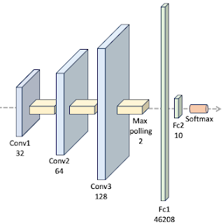
There are various proposed architectures for the training and testing against MNIST data set [ref 2]. We select a 3 layer convolutional neural network followed by two feed forward networks as illustrated below:
We utilize the standard network layer configuration for processing the MNIST dataset.
The ConvNet class is implemented as a PyTorch module [ref 3], handling the model's specification, training, and evaluation. Since the activation function is the sole parameter under evaluation in this study, it is provided as a callable function argument in the constructor.
Each digit is represented as a label in this classification model.
class ConvNet(nn.Module):
    num_classes = 10

def __init__( self, activation: Callable[[torch.Tensor], torch.Tensor]) -> None:
super(ConvNet, self).__init__()
         # Convolutional layers
        self.conv1 = nn.Conv2d(in_channels=1,
out_channels=32, kernel_size=3, stride=1)
self.bn1 = nn.BatchNorm2d(32) self.conv2 = nn.Conv2d(in_channels=32, out_channels=64, kernel_size=3, stride=1)
self.bn2 = nn.BatchNorm2d(64) self.conv3 = nn.Conv2d(in_channels=64, out_channels=128, kernel_size=3, stride=1) self.bn3 = nn.BatchNorm2d(128)
# Drop out shared by all layers self.dropout = nn.Dropout(0.15)
        # Fully connected layers
        in_fc = 46208
        self.fc1 = nn.Linear(in_features=in_fc,
                                       out_features=128)
        self.fc2 = nn.Linear(in_features=128,
out_features=ConvNet.num_classes)
         # Activation function shared by all layers
        self.activation = activation
.
For the sake of simplicity, the various layers of the model share the same dropout (regularization) factor and activation function. The forward method implements the flow of data through the 3 convolutional blocks (convolution, batch normalization, max pooling, activation and drop out.
def forward(self, x: torch.Tensor) -> torch.Tensor:
    # First conv block
    x = self.conv1(x)
    x = self.bn1(x)
    x = F.max_pool2d(x, kernel_size=2)
    x = self.activation(x)
    x = self.dropout(x)

    # Second conv block
    x = self.conv2(x)
    x = self.bn2(x)
    x = F.max_pool2d(x, kernel_size=2)
    x = self.activation(x)
    x = self.dropout(x)

    # Third conv block
    x = self.conv3(x)
    x = self.bn3(x)
    x = F.max_pool2d(x, kernel_size=2)
    x = self.activation(x)
    x = self.dropout(x)

    x = torch.flatten(x, 1)
    # First FFNN block
    x = self.fc1(x)
    x = self.activation (x)

    # Last layer with soft max for output [0, 1]
    x = self.fc2(x)
    return F.log_softmax(x, dim=1)
Training and evaluation are performed with the following hyper-parameters:
- Optimizer: Adam
Learning rate: 0.006
Momentum: 0.89
- Batch size: 32
- Num of epochs: 10
- train to eval ratio: 0.92
- Normal weight initialization: Disabled
- Loss function: Cross entropy
Learning rate: 0.006
Momentum: 0.89
- Batch size: 32
- Num of epochs: 10
- train to eval ratio: 0.92
- Normal weight initialization: Disabled
- Loss function: Cross entropy
The reference implementation of the training and evaluation of the convolutional network in PyTorch is shown in the Appendix.
Evaluation
We compare the following four activation functions:
- Rectified linear unit
- Leaky rectified linear unit
- Exponential linear unit
- Gaussian error linear unit
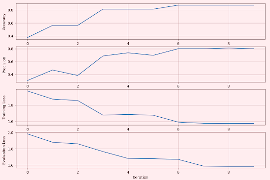
We record and plot the accuracy, precision, training and evaluation loss for the models associated with these activation functions.
Rectified Linear Unit
The Rectified Linear Unit (ReLU), is a widely used activation function in neural networks. It introduces non-linearity into the model, enabling it to learn complex patterns.
Fig. 2 Metrics for Convolutional Network using Rectified Linear Unit - MNIST
Leaky Rectified Linear Unit
Leaky ReLU is a variant of the Rectified Linear Unit (ReLU) activation function used. It address the "dying ReLU" problem, where neurons can stop learning if they consistently output zero. Leaky ReLU introduces a small, non-zero gradient for negative input values, allowing neurons to remain active even when receiving negative inputs.
We use a negative slope of 0.002
Fig. 3 Metrics for Convolutional Network using Leaky Rectifier Linear Unit - MNIST
Exponential Linear Unit
Fig. 4 Metrics for Convolutional Network using Exponential Linear Unit - MNIST
Gaussian Error Linear Unit
The Gaussian Error Linear Unit (GELU) is an activation function popular in transformer architectures (such as BERT and other NLP models)
Fig. 5 Metrics for Convolutional Network using Gaussian Error Linear Unit - MNIST
Analysis
Let's compare the impact of then 4 activation functions on F1 score and evaluation loss.
Fig 6 Impact of selection of activation functions on F1 score for MNIST dataset
The model using exponential linear unit is the only one which F1 score converges quickly to 1.0. All other models have a F1 score of 0.84-0.85. As expected the model ReLU is the slowest to converge.
Fig 7 Impact of selection of activation functions on evaluation loss for MNIST dataset
The loss function profile for the test dataset of each model reflects the previous F1 score plot: the exponential linear unit shows the lowest loss, while the other three models converge toward a similar loss value. ReLU exhibits the slowest convergence profile.
Thanks for reading. For comprehensive topics on geometric learning, including detailed analysis, reviews and exercises, subscribe to Hands-on Geometric Deep Learning
References
[1] MNIST database
[2] Deep Learning Chap 9 Convolutional Networks - I Goodfellow, Y. Bengio, A. Courville - The MIT Press, Cambridge, MA - 2016
[3] Deep Learning with PyTorch Chap 8. Using convolutions to generalize - E. Stevens, L Antiga, T. Viehmann - Manning Publishing, Shelter Island, NY - 2020
-------------
Patrick Nicolas has over 25 years of experience in software and data engineering, architecture design and end-to-end deployment and support with extensive knowledge in machine learning.
He has been director of data engineering at Aideo Technologies since 2017 and he is the author of "Scala for Machine Learning", Packt Publishing ISBN 978-1-78712-238-3 and Geometric Learning in Python Newsletter on LinkedIn.
Appendix
The typical execution of the training and evaluation of the model is implemented by the '__call__' dunda method.
def __call__(self,
             train_loader: DataLoader,
             test_loader: DataLoader,
             output_file_name: Optional[AnyStr] = None) ->
torch.manual_seed(42)
    initialize_weight(list(model.modules()))

   # Train and evaluation process
   for epoch in range(epochs):
      # Set training mode and execute training
      train_loss = self.__train(epoch, train_loader)
      # Set mode and execute evaluation
      eval_metrics = self.__eval(epoch, test_loader)
Here is a basic implementation of the training function commonly used in PyTorch, for reference.
def __train(self, epoch: int, train_loader: DataLoader) -> float:
   total_loss = 0.0
   # Initialize the gradient for the optimizer
   loss_function = nn.CrossEntropyLoss()
   optimizer = optim.Adam(model.parameters(), learning_rate)

   for features, labels in tqdm(train_loader):
      model.train()
      # Reset the gradient to zero
      for params in model.parameters():
params.grad = None
         predicted = model(features)  # Call forward - prediction
         raw_loss = loss_function(predicted, labels)
         logging.info(f'Epoch: {epoch} Loss: {raw_loss}')

         raw_loss.backward(retain_graph=True )
         total_loss += raw_loss.data
         optimizer.step()

   return total_loss / len(train_loader)
The implementation of the evaluation of the model includes the update and collection of metrics to be plotted.
def __eval(self, epoch: int, test_loader: DataLoader) -> Dict[AnyStr, float]:
   total_loss = 0
   loss_func = nn.CrossEntropyLoss()
   metric_collector = {}

   # No need for computing gradient for evaluation
   with torch.no_grad():
      for features, labels in tqdm(test_loader):

         model.eval()
         predicted = model(features)
         p = predicted.cpu().numpy()
         l = labels.cpu().numpy()
for key, metric in metrics.items(): value = metric(p, l) metric_collector[key] = value loss = loss_func(predicted, labels) total_loss += loss.data return metric_collector


No comments:
Post a Comment
Note: Only a member of this blog may post a comment.