I delve into a diverse range of topics, spanning programming languages, machine learning, data engineering tools, and DevOps. Our articles are enriched with practical code examples, ensuring their applicability in real-world scenarios.

Showing posts with label Machine learning. Show all posts
Showing posts with label Machine learning. Show all posts
Tuesday, February 11, 2025

Monday, February 10, 2025
Graph Neural Network Data Loaders
Target audience: Beginner
Estimated reading time: 8'
The versatility of graph representations makes them highly valuable for solving a wide range of problems, each with its own unique data structure. However, generating universal embeddings that apply across different applications remains a significant challenge.
PyTorch Geometric (PyG) simplifies this process by encapsulating these complexities into specialized data loaders, while seamlessly integrating with PyTorch's existing deep learning modules.
PyTorch Geometric (PyG) simplifies this process by encapsulating these complexities into specialized data loaders, while seamlessly integrating with PyTorch's existing deep learning modules.

Table of Contents
What you will learn: How graph data loaders influence node classification in a Graph Neural Network implemented with PyTorch Geometric.
Notes:
- Environments: python 3.12.5, matplotlib 3.9, numpy 2.2.0, torch 2.5.1, torch-geometric 2.6.1
- Source code is available on GitHub [ref 1]
- To enhance the readability of the algorithm implementations, we have omitted non-essential code elements like error checking, comments, exceptions, validation of class and method arguments, scoping qualifiers, and import statement
Introduction
Graph Neural Networks
Data on manifolds can often be represented as a graph, where the manifold's local structure is approximated by connections between nearby points. GNNs and their variants (like Graph Convolutional Networks (GCNs)) extend neural networks to process data on non-Euclidean domains by leveraging the graph structure, which may approximate the underlying manifold [ref 2].
The list of application of graph neural networks includes
- Social Network Analysis – Modeling relationships and community detection.
- Molecular Graphs (Drug Discovery) – Predicting molecular properties.
- Recommendation Systems – Graph-based collaborative filtering.
- Knowledge Graphs – Embedding relations between entities.
- Computer Vision & NLP – Scene graphs, dependency parsing.
For more information, Graph Neural Networks are the topics of a previous article [ref 3]
PyG (PyTorch Geometric)
PyTorch Geometric (PyG) is a graph deep learning library built on PyTorch, designed for efficient processing of graph-structured data. It provides essential tools for building, training, and deploying Graph Neural Networks (GNNs) [ref 4].
The key Features of PyG are:
- Efficient Graph Processing to optimize memory and computation using sparse graph representations.
- Flexible GNN Layers that includes GCN, GAT, GraphSAGE, GIN, and other advanced architectures.
- Batching for Large Graphs to support mini-batching for handling graphs with millions of edges.
- Seamless PyTorch Integration with full compatibility with PyTorch tensors, autograd, and neural network modules.
- Diverse Graph Support for directed, undirected, weighted, and heterogeneous graphs.
The most important PyG Modules are:
- torch_geometric.data to manages graph structures, including nodes, edges, and features.
- torch_geometric.nn to provide data scientists prebuilt GNN layers like convolutional and gated layers.
- torch_geometric.transforms to pre-process input data (e.g., feature normalization, graph sampling).
- torch_geometric.loader to handle large-scale graph datasets with specialized loaders.
Important Note:
This article focuses exclusively on data loaders. Future articles will cover data processing, training, and inference of Graph Neural Networks (GNNs).
Graph Data Loaders
Overview
Some real-world applications involve handling extremely large graphs with thousands of nodes and millions of edges, posing significant challenges for both machine learning algorithms and visualization.
Fortunately, PyG (PyTorch Geometric) enables data scientists to batch nodes or edges, effectively reducing computational overhead for training and inference in graph-based models.
First we need to introduce the attributes of the data of type torch_geometric.data.Data that underline the representation of a graph in PyG.

Table 1. Attributes of graph data in PyTorch Geometric
Data Splits
The graph is divided into training, validation, and test datasets by assigning train_mask, val_mask, and test_mask attributes to the original `Data` object, as demonstrated in the following code snippet.
# 1. Define the indices for training, validation and test data points
train_idx = torch.tensor([0, 1, 2, 4, 6, 7, 8, 11, 12, 13, 14])
val_idx = torch.tensor([3, 9, 14])
test_idx = torch.tensor([5, 10])

#2. verify all indices are accounted for with no overlap
validate_split(train_idx, val_idx, test_idx)

#3. Get the training, validation and test data set
train_data = data.x[train_idx], data.y[train_idx]
val_data = data.x[val_idx], data.y[val_idx]
test_data = data.x[test_idx], data.y[test_idx]
Alternatively, we can use the RandomNodeSplit and RandomLinkSplit classes to directly extract the training, validation, and test datasets.
from torch_geometric.transforms import RandomNodeSplit

transform = RandomNodeSplit(is_undirected=True)
train_data, val_data, test_data = transform(data)
Common Loader Architectures
The graph nodes and link loaders are an extension of PyTorch ubiquitous data loader. A node loader performs a mini-batch sampling from node information and a link loader performs a similar mini-batch sampling from link information.'
The latest version of PyG supports an extensive range of graph data loaders. Below is an illustration of the most commonly used node and link loaders..
Random node loader
A data loader that randomly samples nodes from a graph and returns their induced subgraph. In this case, the two sampled subgraphs are highlighted in blue and red.
Class: RandomNodeLoader

Fig 1. Visualization of selection of graph nodes in a Random node loader
Neighbor node loader
This loader partitions nodes into batches and expands the subgraph by including neighboring nodes at each step. Each batch, representing an induced subgraph, starts with a root node and attaches a specified number of its neighbors. This approach is similar to breath-first search in trees.
class NeighborLoader

Fig 2. Visualization of selection of graph nodes in a Neighbor node loader
Neighbor link loader
This loader is similar to the neighborhood node loader. It partitions links and associated nodes into batches and expands the subgraph by including neighboring nodes at each step
Class LinkNeigbhorLoader

Fig 3. Visualization of selection of graph nodes in a Neighbor link loader
Subgraphs Cluster
Divides a graph data object into multiple subgraphs or partitions. A batch is then formed by combining a specified number (`batch_size`) of subgraphs. In this example, two subgraphs, each containing five green nodes, are grouped into a single batch.
Class ClusterData

Fig 4. Visualization of selection of graph nodes in a cluster loader
Graph Sampling Based Inductive Learning Method
This is an inductive learning approach that enhances training efficiency and accuracy by constructing mini-batches through sampling subgraphs from the training graph, rather than selecting individual nodes or edges from the entire graph. This approach is similar to depth-first search in trees.
Classes: GraphSAINTNodeSampler, GraphSAINTRandomWalkSampler

Fig 5. Visualization of selection of graph nodes in a Graph SAINT random walk
Evaluation
Let's analyze the impact of different graph data loaders on the performance of a Graph Convolutional Neural Network (GCN).
To facilitate this evaluation, we'll create a wrapper class, `GraphDataLoader`, for managing data loading. The `__call__` method directs requests to the appropriate node or link sampler/loader, with an optional num_workers parameter for parallel processing.
The arguments of the constructor are:
- loader_attributes: Dictionary for the configuration of this specific loader
- data: The graph data of type torch_geometric.data.Data
# --- Code Snippet 1 ---
     from torch_geometric.data import Data
from torch.utils.data import DataLoader
from torch_geometric.loader import (NeighborLoader, RandomNodeLoader,
GraphSAINTRandomWalkSampler, GraphSAINTNodeSampler, GraphSAINTEdgeSampler, ShaDowKHopSampler, ClusterData, ClusterLoader)
from networkx import Graph
class GraphDataLoader(object):
def __init__(self,
loader_attributes: Dict[AnyStr, Any],
data: Data) -> None:
self.data = data
self.attributes_map = loader_attributes
# Routing to the appropriate loader given the attributes dictionary
    def __call__(self, num_workers: int) -> (DataLoader, DataLoader):
        match self.attributes_map['id']:
            case 'NeighborLoader':
                return self.__neighbors_loader()
            case 'RandomNodeLoader':
                return self.__random_node_loader()
            case 'GraphSAINTNodeSampler':
                return self.__graph_saint_node_sampler()
            case 'GraphSAINTEdgeSampler':
                return self.__graph_saint_edge_sampler()
            case 'ShaDowKHopSampler':
                return self.__shadow_khop_sampler()
            case 'GraphSAINTRandomWalkSampler':
                return self.__graph_saint_random_walk(num_workers)
            case 'ClusterLoader':
                return self.__cluster_loader()
            case _:
                raise DatasetException(f'Data loader {self.attributes_map["id"]} not supported')
To keep this article concise, our evaluation focuses on the following three graph data loaders:
- Random Nodes
- Neighbors Nodes
- Graph SAINT Random Walk
Random Node Loader
The only configuration attribute for the random node loader is num_parts that controls how the dataset is partitioned into smaller chunks for efficient sampling. The data set is split into num_parts subgraphs to improve performance and parallelization for large graphs. We use the default batch_size 128.
The loader for the training set shuffles the data while the order of data points for the validation set is preserved.
# --- Code Snippet 2 ---
     def __random_node_loader(self) -> (DataLoader, DataLoader):
   num_parts = self.attributes_map['num_parts']
   train_loader = RandomNodeLoader(self.data, num_parts=num_parts, shuffle=True)
val_loader = RandomNodeLoader(self.data, num_parts=num_parts, shuffle=False) return train_loader, val_loader
We consider the Flickr data set included in Torch Geometric (PyG) described in [ref 5]. As a reminder, The Flickr dataset is a graph where nodes represent images and edges signify similarities between them [ref 6]. It includes 89,250 images and 899,756 relationships. Node features consist of image descriptions and shared properties.
T. The purpose is to classify Flickr images (defined as graph nodes) into one of the 108 categories.
I # --- Code Snippet 3 ---
     import os
from torch_geometric.datasets.flickr import Flickr
import torch_geometric
# Load the Flickr data set then extract the first and only graph data # from the dataset
path = os.path.join(os.path.dirname(os.path.realpath(__file__)), '..', 'data', 'Flickr')
_dataset: Dataset = Flickr(path)
_data: torch_geometric.data.data.Data = _dataset[0]
# Define the appropriate attribute for this loader: Random nodes
attrs = {
'id': 'RandomNodeLoader',
'num_parts': 256
}
graph_data_loader = GraphDataLoader(loader_attributes= attrs, data=_data)
# Invoke of generic __call__
train_data_loader, test_data_loader = graph_data_loader()
We train a three-layer message-passing Graph Convolutional Neural Network (GCN) on the Flickr dataset for classify these images into 108 categories. In this first experiment the model trains on data extracted by the random node loader. For clarity, the code for training the model, computing losses, and evaluating performance metrics has been omitted.
The following plot tracks the various performance metrics (accuracy, precision and recall) as well as the training and validation loss over 60 iterations.
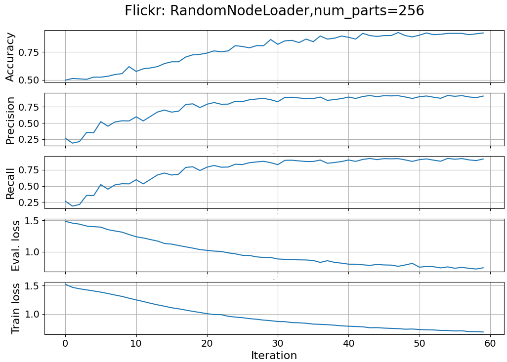
Fig 6. Performance metrics and loss for a GCN in a multi-label classification of data loaded randomly
Neighbor Node Loader
The configuration parameters used for this loader include:
- num_neighbors: Specifies the number of neighbors to sample at each layer or hop in a Graph Neural Network. It is defined as an array, e.g., `[num_neighbors_first_hop, num_neighbors_second_hop, ...]`.
- replace: Determines whether sampling is performed with or without replacement.
- batch_size; Size of the batch
We specify few other parameters which value do not vary during our evaluation>
- drop_last: to drop the last batch is it is less that the prescribed batch_size
- input_nodes for the applying the mask for training and validation data
# --- Code Snippet 4 ---
     def __neighbors_loader(self) -> (DataLoader, DataLoader):
     # Extract loader configuration
   num_neighbors = self.attributes_map['num_neighbors']
   batch_size = self.attributes_map['batch_size']
   replace = self.attributes_map['replace']

    # Generate the loader for training data
    train_loader = NeighborLoader(self.data,
                                                     num_neighbors=num_neighbors,
                                                     batch_size=batch_size,
                                                     replace=replace,
                                                     drop_last=False,
                                                     shuffle=True,
                                                     input_nodes=self.data.train_mask)

        # Generate the loader for validation data
    val_loader = NeighborLoader(self.data,
                                                   num_neighbors=num_neighbors,
                                                   batch_size=batch_size,
                                                   replace=replace,
                                                   drop_last=False,
                                                   shuffle=False,
                                                   input_nodes=self.data.val_mask)
return train_loader, val_loader
We only need to update the dictionary of this loader configuration parameters in the code snippet 3.
# --- Code Snippet 5 ---
    attrs = {
      'id': 'NeighborLoader',
      'num_neighbors': [6, 4],
      'batch_size': 1024,
      'replace': True
}
The training and validation of the Graph Convolutional Neural Network produces the following plots for the performance metrics and losses.

Fig 7. Performance metrics and loss for a GCN in a multi-label classification of data loaded with a Neighbor loader
Graph Sampling Based Inductive Learning loader
For evaluating this loader, we use the following configuration parameters:
- walk_length: Defines the number of hops (nodes) in a single random walk
- batch_size: Size of the batch of subgraph
- num_steps: Number of times new nodes are samples in each epoch
- sample_coverage: Number of times each node is sampled: appeared in a batch.
                          # --- Code Snippet 6 ---

def __graph_saint_random_walk(self,
                                                          num_workers: int) -> (DataLoader, DataLoader):

        # Dynamic configuration parameter for the loader
     walk_length = self.attributes_map['walk_length']
     batch_size = self.attributes_map['batch_size']
     num_steps = self.attributes_map['num_steps']
     sample_coverage = self.attributes_map['sample_coverage']

        # Extraction of the loader for training data
     train_loader = GraphSAINTRandomWalkSampler(data=self.data,
                                                   batch_size=batch_size,
                                                   walk_length=walk_length,
                                                   num_steps=num_steps,
                                                   sample_coverage=sample_coverage,
                                                   shuffle=True)

        # Extraction of the loader for validation data
     val_loader = GraphSAINTRandomWalkSampler(data=self.data,
                                                 batch_size=batch_size,
                                                 walk_length=walk_length,
                                                 num_steps=num_steps,
                                                 sample_coverage=sample_coverage,
                                                 shuffle=False)
   return train_loader, val_loader
Once again, we reuse the implementation in code snippet 3 and update the dictionary of this loader configuration parameters.
                        # --- Code Snippet 7 ---

attrs = {
     'id': 'GraphSAINTRandomWalkSampler',
'walk_length': 3,
'num_steps': 12,
'sample_coverage': 100,
'batch_size': 4096
}

Fig 8. Performance metrics and loss for a GCN in a multi-label classification of data loaded with a Graph SAINT random walk loader
The performance metrics, accuracy, precision and recall points to an inability for the Random walk to capture long-range dependencies.
Comparison
Lastly, let's compare the impact of each data loader on the precision of the graph convolutional neural network..

Fig 9. Plotting precision in a multi-label classification of a GCN with various graph data loaders
Although the random walk for the GraphSAINTRandomWalk loader excels in analyzing and representing local structure, it fails to capture the global context (high number of hops - dependencies) of a large image set. Moreover, the plot highlights the high degree of instability of performance metrics even though the loss in the validation run converges appropriately.
NeighborNodeLoader select nodes across multiple hops and therefore avoid over emphasis on nodes sampled in nearby regions.
Here is a summary of benefits, drawbacks and applicability of the 3 graph data loaders.

Table 2. Pros and cons of Random node, Neighbor node and Random walk loaders
Monday, December 16, 2024
Reviews of Papers on Geometric Learning - 2024
 '
'- ChatGPT for Computational Topology
- An introduction to Topological Data Analysis
- Synthetic Data Generation and Deep Learning for the Topological Analysis of 3D Data
- Deep Learning Symmetries and Their Lie Groups, Algebras, and Subalgebras from First Principles
- Autoencoders for discovering manifold dimension and coordinates in data from complex dynamical systems
- Reliable Malware Analysis and Detection using Topology Data Analysis
- Algebra, Topology, Differential Calculus, and Optimization Theory For Computer Science and Machine Learning
- Categorical Foundations of Explainable AI
- Introduction to Geometric Learning in Python with Geomstats
- Machine Learning Algebraic Geometry for Physics
- Deep Learning in Asset Pricing
- Intrinsic and extrinsic deep learning on manifolds
- Kalman Filters on Differentiable Manifolds
- Manifold Matching via Deep Metric Learning for Generative Modeling
- Machine learning a manifold
- A Geometric Perspective on Variational Autoencoders
- Deep Hyperspherical Learning
- Learning Weighted Submanifolds with Variational Autoencoders and Riemannian Variational Autoencoders
- Learning Manifold Dimensions with Conditional Variational Autoencoders
- Variational Transformer Autoencoder with Manifolds Learning
- Riemannian Score-Based Generative Modelling
- Riemannian Diffusion Models
- Convolutional Neural Networks on Manifolds: From Graphs and Back
- Riemannian Residual Neural Networks
- A singular Riemannian geometry approach to Deep Neural Networks
- Transformer with Hyperbolic Geometry
- Deep Extrinsic Manifold Representation for Vision Tasks
- Manifold Matching via Deep Metric Learning for Generative Modeling
- Pullback Flow Matching on Data Manifolds
- A Survey of Geometric Optimization for Deep Learning: From Euclidean Space to Riemannian Manifold
The purpose of the study is to enable ChatGPT to support theoretical mathematicians in the creation of algorithms and code, bypassing the need for deep programming language expertise.
Through dialogue with ChatGPT, mathematicians can impart their knowledge of mathematical concepts and theories in simple English. ChatGPT would then use this guidance to convert the mathematical theories into executable algorithms and code, eliminating the necessity for mathematicians to be versed in the intricacies of coding.
The paper concentrates on directing ChatGPT to produce Python code, utilizing the 'networkx' and 'scipy' libraries, for several tasks:
- Computing Betti numbers for a simplicial complex
- Constructing a Vietoris-Rips complex
- Creating a boundary matrix for a specified simplicial complex
- Formulating a graph Laplacian matrix.
2. An introduction to Topological Data Analysis
This article provides a comprehensive yet concise guide to applying Topological Data Analysis (TDA) in data analysis, offering just enough information without overwhelming the reader. TDA is a burgeoning field that utilizes novel tools from algebraic topology and computational geometry to extract significant features from complex data sets.
What I appreciate about the paper is
- Clear definition of the TDA pipeline, which interestingly doesn't rely on Euclidean metrics.
- Its accessibility to non-experts, introducing fundamental TDA concepts like metric spaces, simplicial complexes, and Persistent homology in an understandable manner (although I feel that the sections on applying persistent homology in data analysis, feature engineering, and optimizing machine learning architectures could have been more detailed and extensive
- The way it illustrates the concept of filtration with practical examples and visual aids
- The application of persistent homology to proteins, demonstrated with Python code and the Gudhi library.
Have you ever pondered whether Neural Networks can be used to determine the manifold topology in 3D data?
This paper provides insights into this query. It introduces Persistent Homology and Betti numbers as tools for comprehending the topology of 3D objects. The paper explains how convolutional neural networks can minimize the computational resources typically needed for applying persistent homology.
Additionally, it explores the application and comparison of various networks for semantic segmentation of topology data, offering an enhanced TDA method. This includes: (1) A transformer block featuring self-attention for 3D point clouds, and (2) a manifold curvature estimator, both yielding similar outcomes.
Much effort in the field of machine learning is devoted to creating increasingly complex models. However, it is becoming evident that the caliber of training and validation data is crucial, aligning with the concept of Data-centric AI.
The paper discusses how defining symmetry properties in the hidden layers of a deep learning model can streamline its training and make it easier to interpret. It introduces a neural network architecture that detects and classifies symmetric patterns in a labeled training dataset.
The paper discusses how defining symmetry properties in the hidden layers of a deep learning model can streamline its training and make it easier to interpret. It introduces a neural network architecture that detects and classifies symmetric patterns in a labeled training dataset.
This method utilizes group theory to:
- Generate symmetry transformations that maintain the integrity of labeled data.
- Pinpoint infinitesimal transformations, known as symmetry generators.
- Modify the machine learning model's loss function to uncover sub-algebras (Lie algebra) of the symmetry group, which are formed as linear combinations of the symmetry generators.
- Ascertain the complete symmetry group and Lie subgroups that optimize the number of generators.
Reducing dimensions, whether implicitly or explicitly, is key to enhancing the prediction accuracy of complex models that handle continuous data. The authors have trained an Autoencoder framework that incorporates regularization. This framework uses multiple internal linear layers and the L2 norm. The precise dimensionality of the feature space is determined by conducting a singular value decomposition on the covariance matrix of the latent Z space in the auto-encoder. This approach combines the best aspects of both methodologies!
The concept was put to the test for identifying 3-dimensional (and in another case, 8-dimensional) manifolds within a 4-dimensional (and respectively, infinite-dimensional) Euclidean space. This was done using data derived from various nonlinear partial differential equations. The outcomes are remarkable: the proposed method uniquely succeeded in pinpointing the top 3 (or 8) singular/eigenvalues, outperforming both PCA and generic Autoencoders.
The concept was put to the test for identifying 3-dimensional (and in another case, 8-dimensional) manifolds within a 4-dimensional (and respectively, infinite-dimensional) Euclidean space. This was done using data derived from various nonlinear partial differential equations. The outcomes are remarkable: the proposed method uniquely succeeded in pinpointing the top 3 (or 8) singular/eigenvalues, outperforming both PCA and generic Autoencoders.
The reader should have basic knowledge of unsupervised, dimension reduction.
The Python code is available on GitHub https://github.com/mdgrahamwisc/IRMAE_WD6. Reliable Malware Analysis and Detection using Topology Data Analysis
This paper introduces and evaluates three topological-based data analysis (TDA) techniques, to efficiently analyze and detect complex malware signature. TDA is known for its robustness under noise and with imbalanced datasets.
The paper first introduces the basic formulation of metric spaces, simplicial complexes, and homology before describing the 3 techniques for analysis.
- TDA mapper
- Persistence homology
- Topological model analysis tool
These TDA techniques are compared to traditional features engineering (unsupervised) algorithms such as PCA or t-SNE using a False Positive Rate and a Detection Rate. The features are then used as input to various traditional ML classifiers (SVM, Logistic Regression, Random Forest, Gradient Boosting,).
The paper also covers CPU and memory usage analysis.
Conclusion:
TDA mapper with PCA for feature extraction for extracting malware clusters as well as t-SNE to identify overlapping malware characteristics.
As far as detection rate in supervised classification, Random Forest, XGBoost and GBM achieve a detection rate close to 100%
Basic understanding of machine learning and algebraic topology is required to benefit from the paper.
I discovered a remarkably thorough review of all the mathematics essential for machine learning. This review is well-articulated, making it accessible even for those less enthusiastic about mathematics (no need to bring out your dissertation). Spanning over 2100 pages, the paper encompasses a wide range of algorithms, from fundamental linear algebra, dual space, and eigenvectors to more advanced topics like tensor algebra, affine geometry, topology, homologies, kernel models, and differential forms.
The structure of the paper allows for independent topic exploration. For instance, you can jump right into the chapter on soft-margin support vector machines without needing to go through the preceding chapters. This makes the paper an invaluable resource for anyone seeking a comprehensive mathematical foundation in machine learning.
The index and bibliography are both extensive and detailed. However, a minor drawback is that the only coding examples provided are in Matlab, with no Python implementations.
8. Categorical Foundations of Explainable AI
Category Theory to Explain Model Prediction
Explainable AI (XAI), a vital research area addressing ethical and legal AI issues, still lacks a solid mathematical foundation. Category theory offers a solution.
This paper starts with an overview of Category theory basics, such as feedback monoids and cartesian streams. It then presents frameworks for Explaining Learning Agents and Agent translators. These concepts are applied to a basic multilayer perceptron using the ADAM optimizer. The study compares model-agnostic explaining formalisms with model-specific ones. It also introduces a forward-based explainer (relying on model parameters) and a backward-based explainer (utilizing the loss function and gradient).
Ultimately, the XAI framework provides a structured definition of explanation and lays the groundwork for classifying explanations both synthetically and semantically.
Linear models sometimes fall short when dealing with high-dimensional data found in areas like computer vision, molecular biology, or radar signal processing. This type of data typically exists on curved, differentiable vector spaces, known as manifolds. Training and validating models with manifold data necessitates the use of differential geometry.
The paper highlights Geomstats, an open-source Python toolkit for handling data on non-linear manifolds. Included in the package are tutorials that combine theoretical concepts with practical Python implementations, such as
- Statistics and Geometric Statistics, demonstrated through hypersphere and Frechet mean examples.
- Techniques for managing Data on Manifolds, utilizing the exponential map (tangent vector) and the Riemann Tensor metric.
- Classifying Symmetric Positive Definite matrices, which allows for the application of standard learning algorithms, like the K-Nearest Neighbors classifier, to non-linear manifolds.
- Graph representations that involve embeddings in hyperbolic spaces.
- This paper serves as an ideal entry point into the world of manifold learning, offering an easy-to-understand overview without requiring deep expertise in differential geometry.
Source code available at github.com/geomstats/geomstats
A quick tutorial is available at https://youtu.be/Ju-Wsd84uG0
10. Machine Learning Algebraic Geometry for Physics
This paper is a valuable contribution to any discussion or teaching on Information Geometry (refer to the mentioned source).
While some are accustomed to applying laws of Physics, like Partial Differential Equations, to restrict deep learning models in machine learning, the use of machine learning combined with algebraic/differential geometry to process large datasets produced by physics is relatively unusual.
The paper utilizes the Calabi-Yau manifold, derived from the string theory concept of a 10-dimensional spacetime landscape. It examines unsupervised models such as PCA, Topology Data Analysis, Clustering, and then explores neural networks used for data analysis on hypersurfaces. The authors delve into a variety of subjects including projecting to lower-dimensional spaces, Hilbert series, interactions, and equivalences of Branes, as well as cluster mutations.
The study concludes by discussing the optimal transport problem and Kahler geometry in the context of Generative Adversarial Networks.
Reference: Information Geometry: Near Randomness and Near Independence - K. Arwini, C.T.J. Dobson – Springer 2008
Deep learning enhances dynamic asset pricing by streamlining the feature engineering process. This approach was tested in an empirical study spanning 40 years and involving 30,000 individual stocks.
Note: This paper is accessible to those without financial expertise and only a basic understanding of deep learning, as the models are explained in clear terms.
The assessment and comparison of various machine learning models were conducted through Monte Carlo Simulations, with Max a Posterior Estimation (MAPE) as objective.
The findings indicate:
A crucial takeaway is the importance of integrating domain-specific knowledge and financial theory into deep learning models to make them both more effective and interpretable.- Predicting stock prices is challenged by significant issues related to distribution and concept shift.
- Advanced deep learning models generally surpass traditional linear predictors in performance.
- Among these, Recurrent Neural Networks, especially LSTM and GRU featuring attention mechanisms and transformers, demonstrate superior effectiveness.
- The addition of skip connections in deep layers did not lead to performance enhancements.
- Convolutional Neural Networks were found to be less effective than even simple feedforward neural networks.
Note: This paper is accessible to those without financial expertise and only a basic understanding of deep learning, as the models are explained in clear terms.
This paper introduces two types of general deep neural network architecture on manifolds:
Extrinsic deep neural network on manifolds
This architecture maintains the geometric characteristics of manifolds by employing an equivariant embeddings of a manifold into the Euclidean space.
This method is applied in regression models or Gaussian processes on manifolds, where the idea is to construct the neural network based on the manifold's representation after embedding, while still maintaining its geometric properties. By adopting this strategy, it becomes possible to utilize stochastic gradient descent and backpropagation techniques from Euclidean space. This results in enhanced accuracy compared to conventional machine learning algorithms like SVM, random forest, etc.
Intrinsic deep neural network on manifolds
The objective is to embed the inherent geometric nature of Riemannian manifolds using exponential and logarithmic maps. This framework, which projects localized points from a Riemannian manifold onto a single tangent space, proves beneficial when embeddings cannot be determined. Each localized tangent space (or chart) is mapped (via exp/log functions) onto a neural network. This architectural approach achieves higher accuracy compared to deep models in Euclidean space and the Extrinsic architecture.
These two frameworks are assessed based on their performance in 1) classifying health-related simulated datasets on a spherical manifold, and 2) dealing with symmetric semi-positive definite matrices.
Extrinsic deep neural network on manifolds
This architecture maintains the geometric characteristics of manifolds by employing an equivariant embeddings of a manifold into the Euclidean space.
This method is applied in regression models or Gaussian processes on manifolds, where the idea is to construct the neural network based on the manifold's representation after embedding, while still maintaining its geometric properties. By adopting this strategy, it becomes possible to utilize stochastic gradient descent and backpropagation techniques from Euclidean space. This results in enhanced accuracy compared to conventional machine learning algorithms like SVM, random forest, etc.
Intrinsic deep neural network on manifolds
The objective is to embed the inherent geometric nature of Riemannian manifolds using exponential and logarithmic maps. This framework, which projects localized points from a Riemannian manifold onto a single tangent space, proves beneficial when embeddings cannot be determined. Each localized tangent space (or chart) is mapped (via exp/log functions) onto a neural network. This architectural approach achieves higher accuracy compared to deep models in Euclidean space and the Extrinsic architecture.
Even though data from real-world control applications are complex and typically reside on manifolds, the Kalman filter has traditionally been developed for Euclidean spaces. This paper presents a more adaptable approach than the widely utilized error-state extended Kalman filter for managing manifold constraints. It showcases a method that incorporates these constraints directly into the Kalman filtering process, using examples of 3-dimensional rotation and motion groups.
The structure of the paper is as follows:
- A concise overview of differentiable manifolds, tangent spaces, and the exponential/logarithmic mappings.
- A discussion on modeling the error state and the covariance matrix.
- A detailed description of how to apply the predict and update steps of the Kalman filter from tangent spaces back to the manifold context.
To demonstrate the practical application of the Error-state Kalman filter on manifolds, a controlled Lidar navigation system is examined.
Note: The reader should have a foundational understanding of differential geometry and Lie algebra to fully grasp the content of this paper.
I would recommend “The SO(3) and SE(3) Lie Algebras of Rigid Body Rotations and Motions and their Application to Discrete Integration, Gradient Descent Optimization, and State Estimation” to get familiar with lie algebras, manifolds and extended Kalman.
This study advances the recent progress in blending geometry with statistics to enhance generative models. It proposes a novel method for identifying manifolds within Euclidean spaces for generative models like variational encoders and GANs through two neural networks:
The metric generator produces a pullback of the Euclidean space while the data generator produces a push forward of the prior distribution. The algorithm is described with easy-to-follow pseudo code.
The method is tested on unconditional ResNet image creation and GAN-based image super-resolution, showing improved Frechet Inception Distance and perception scores.
This paper will be especially of interest to engineers already familiar with GANs and Frechet metric.
- Data generator sampling data on the manifold
- Metric generator learning geodesic distances.
The metric generator produces a pullback of the Euclidean space while the data generator produces a push forward of the prior distribution. The algorithm is described with easy-to-follow pseudo code.
The method is tested on unconditional ResNet image creation and GAN-based image super-resolution, showing improved Frechet Inception Distance and perception scores.
This paper will be especially of interest to engineers already familiar with GANs and Frechet metric.
In quantum physics, the symmetry of experimental data often simplifies many challenges. The researchers utilize neural networks to detect symmetries within a dataset. They define a symmetry V in the context of a transformation f acting on coordinates X within a manifold, where V(x) = V(f(x)). This approach focuses on the manifold's local properties, which helps manage issues arising from data with very high dimensions, as the Lie algebra is situated within the manifold's tangent space.
To achieve this, an 8-layer feed-forward network is employed for interpolating data, predicting infinitesimally transformed fields, and identifying the symmetry. The Keras library is used for this implementation. The neural model is capable of recognizing symmetries in the Lie groups of SU(3), which involves orientation preservation, and SO(8), which relates to Riemannian metric invariance.
Understanding this paper benefits from some background in differential geometry, Lie algebra, and manifolds.
For introduction to manifolds, as reference: https://math.berkeley.edu/~jchaidez/materials/reu/lee_smooth_manifolds.pdf
To achieve this, an 8-layer feed-forward network is employed for interpolating data, predicting infinitesimally transformed fields, and identifying the symmetry. The Keras library is used for this implementation. The neural model is capable of recognizing symmetries in the Lie groups of SU(3), which involves orientation preservation, and SO(8), which relates to Riemannian metric invariance.
Understanding this paper benefits from some background in differential geometry, Lie algebra, and manifolds.
Variational autoencoders (VAEs) are generative models that encode input data into a reduced-dimensional latent space, making them well-suited for manifold modeling. In a standard VAE, the latent space's multivariate Gaussian distribution is substituted with a uniform distribution on the manifold, employing the Riemannian tensor metric. This Riemannian metric in the latent space is approximated using a first-order Taylor series, known as a pull-back metric.
This modeling approach enables sampling of latent values for datasets like MNIST, CIFAR, and CELEBA. These samples are then assessed against a range of autoencoders, from Wasserstein to Hamiltonian, using evaluation metrics such as Frechet Inception Distance (FID) and Precision/Recall (PRD) – specifically, F1 scores.
This modeling approach enables sampling of latent values for datasets like MNIST, CIFAR, and CELEBA. These samples are then assessed against a range of autoencoders, from Wasserstein to Hamiltonian, using evaluation metrics such as Frechet Inception Distance (FID) and Precision/Recall (PRD) – specifically, F1 scores.
The sampling VAE that utilizes the manifold model demonstrates a marked enhancement in FID and PRD for the CIFAR10 and CELEBA datasets.
This study addresses certain limitations of convolutional neural networks (CNNs) during training, such as overfitting and vanishing gradients. The suggested approach involves:
- Incorporating a geometric constraint by substituting the Euclidean inner product with the geodesic distance on a hypersphere.
- Replacing the softmax loss with a normalized softmax loss that is weighted by a metric tensor (dependent on the geodesic distance input and convolution weights) on the hypersphere.
The model's performance was assessed using the CIFAR-10/100 and ImageNet-2012 datasets, without ReLU activation, and compared to the ResNet-32 model. The proposed model achieves an accuracy comparable to the most efficient ResNet model but converges significantly faster.
18. Learning Weighted Submanifolds with Variational Autoencoders and Riemannian Variational Autoencoders
A great paper from Nina Miolane, one of the contributors of Geomstats, a very useful Python library for Geometric learning.
The author explores alternative to Euclidean data representation, motivated by the brain connectomes in MRI and devise a Riemannian variational autoencoder (with latent space as a Manifold or Lie group).
The paper evaluates geodesic vs. non-geodesic subspaces, review the standard Euclidean variational autoencoder, introduces Riemannian VAE including maximization of a modified Evidence Lower Bound. The generative function applied to latent space is constructed from the Euclidean version through the Riemannian exponential map at the base point on the manifold. The model is evaluating using a 2-Wassertein distance on S3 and H2 groups/manifolds.
The authors seek to determine the dimension of the underlying manifold—a geometric characteristic—from the global minimum of a variational autoencoder (VAE) setup that includes an encoder, a decoder, and a Gaussian distribution prior.
The study highlights several trade-offs in the design of autoencoders, with these key findings:
- A conditioned prior is unnecessary: a normal distribution prior suffices.
- The initial variance of the Gaussian decoder impacts the loss function.
- Commonly used strategies like weight sharing to accelerate training may hinder convergence.
The evaluation of both Variational Autoencoders (VAE) and Conditional Variational Autoencoders (CVAE) was conducted using the standard ELBO metrics across three datasets:
- A synthetic dataset with 5-dimensional categorical data, consisting of 100,000 samples.
- The MNIST dataset implemented with ResNet blocks.
- The Fashion MNIST dataset.
The results indicate that the correct number of active dimensions were identified (5 for the synthetic dataset and 20 for MNIST), provided that the latent dimension was sufficiently large.
20. Variational Transformer Autoencoder with Manifolds Learning
The paper illustrates how the Riemann metric effectively addresses the challenges of modeling non-linear latent spaces by interpolating between input data samples along geodesics. The researchers have developed a variational autoencoder that incorporates a spatial transformer as the encoder to map the latent space model onto a Riemann manifold.
The paper illustrates how the Riemann metric effectively addresses the challenges of modeling non-linear latent spaces by interpolating between input data samples along geodesics. The researchers have developed a variational autoencoder that incorporates a spatial transformer as the encoder to map the latent space model onto a Riemann manifold.
The goal is to refine the variational auto-encoder to calculate the geodesic distances between input data points, utilizing the Riemann metric tensor, and to delineate a semantic feature/latent space. The encoded transformer component is responsible for calculating the prior in the latent space. Importantly, this new model does not necessitate any modifications to the existing loss function (ELBO) or the training methodology.
Implemented in PyTorch, the model consists of four convolutional layers, two linear reshaping layers, and fifty latent variables. It has been evaluated using a variety of image sets, including grayscale images (such as MNIST and FashionMNIST) and color, natural images (such as CelebA and CIFAR-10). The proposed model demonstrates substantial improvements in image reconstruction.
Note: The paper assumes knowledge of differential geometry and generative models. The source code is available on GitHub.
21. Riemannian Score-Based Generative Modelling
Diffusion models, or score-based generative models, progressively add noise to create a generative model that reverses the noise addition process over time. Although effective, these models primarily utilize data in Euclidean space and often fail to capture the intrinsic geometry of complex data such as proteins, geological formations, or high-energy physics components.
This paper outlines four steps to adapt diffusion models to manifolds:
Diffusion models, or score-based generative models, progressively add noise to create a generative model that reverses the noise addition process over time. Although effective, these models primarily utilize data in Euclidean space and often fail to capture the intrinsic geometry of complex data such as proteins, geological formations, or high-energy physics components.
- Modify the noise addition process to suit manifolds using the Riemannian gradient.
- Incorporate Brownian motion into the Euclidean time-reversal formula.
- Implement Geodesic random walks to approximate sampling from stochastic differential equations.
- Approximate and evaluate the drift in the time-reversal process.
Code is available on Github.
22. Riemannian Diffusion Models
Euclidean diffusion models often fail to capture the generative factors related to the geometry of the space in applications such as protein modeling or geoscience. This paper introduces a variational architecture for the Riemann manifold, applying the Feynman-Kac conditional expectation to the Ito-diffusion process.
The authors address the diffusion stochastic differential equation on the manifold by defining test functions within a variational framework based on the Riemannian divergence of vector fields (Evidence Lower Bound). The proposed solution is validated by its association with the Riemannian score-based model, replicating the same relationship found in Euclidean space.
The algorithm is evaluated on various manifolds, including Hyperbolic spaces, SO(n), Tori, and Hyperspheres. Notably, the authors include an appendix reviewing key elements of differential geometry for non-experts.
The algorithm is evaluated on various manifolds, including Hyperbolic spaces, SO(n), Tori, and Hyperspheres. Notably, the authors include an appendix reviewing key elements of differential geometry for non-experts.
23. Convolutional Neural Networks on Manifolds: From Graphs and Back
This paper extends deep learning models to non-Euclidean spaces by introducing manifold convolution filters. The convolutional neural network is constructed by stacking convolution layers based on Laplace-Beltrami (LB) operators for the heat diffusion process.
This paper extends deep learning models to non-Euclidean spaces by introducing manifold convolution filters. The convolutional neural network is constructed by stacking convolution layers based on Laplace-Beltrami (LB) operators for the heat diffusion process.
After presenting the fundamental concepts of manifold signals and intrinsic gradients, the authors explore sequentially:
- The extraction of orthogonal eigenvalues from the LB operator
- The definition of the manifold filter and its frequency response using eigenfunctions
- The assembly of a bank of filters into a manifold neural network
- The sampling of space and time domains to approximate a continuous architecture with point clouds
- The discretization of the filter by reformulating the LB operator as a graph Laplacian
24. Riemannian Residual Neural Networks
This paper introduces the extension of residual neural networks to Riemannian manifolds.
Residual Neural Networks
Residual networks were initially designed to mitigate the issues of vanishing and exploding gradients in deep neural networks. These networks achieve this by learning residual functions relative to the layer inputs using identity mappings.
Riemannian Residual Neural Networks
The primary aim of this paper is to extend residual neural networks to Riemannian manifolds. By leveraging Riemannian geometry concepts such as tangent spaces, induced metrics, geodesics, and pullback/pushforward techniques, the paper demonstrates how to represent residuals and outputs from each hidden layer of a neural network on manifolds with constant sectional curvature, including Euclidean, Hyperbolic, and Spherical spaces.
Projection and Implementation
The authors detail the method of projecting the residuals for each hidden layer from the local Euclidean tangent space onto manifold geodesics via the exponential map. The implementation focuses on hyperplanes and uses the Whitney embedding theorem to project vector fields onto the tangent space. The feature map, induced by these vector fields, is learned through a pullback mechanism, assuming a closed-form definition for the exponential map.
Performance
The Riemannian residual networks show superior performance compared to various graph neural network variants on manifolds with semi-defined positive matrices.
25. A singular Riemannian geometry approach to Deep Neural Networks
manifolds, with a Riemannian metric applied to the final layer. This metric is propagated back through the layers or maps.
The authors' approach includes:
- Reviewing essential elements of Riemannian geometry.
- Defining the geometry for smooth layers (utilizing weights, biases, and activation functions) and for the entire smooth network (considered as a sequence of maps between manifolds).
- Applying this framework to analyze the equivalence of neural networks in classification problems, focusing on representation within the input manifold.
- Evaluating level curves and equivalence classes for non-linear regression, demonstrated with the Ackley function.
- Studying the space of weights and biases for a given input.
26. Transformer with Hyperbolic Geometry
The paper presents a novel transformer architecture that leverages both hyperbolic and Euclidean spaces. It incorporates a hyperbolic-to-linear transformation within the self-attention module.
To address performance degradation in high-dimensional settings, the authors generate hyperbolic keys and queries. They use the Poincaré ball with negative Riemannian curvature as the hyperbolic representation, projecting from the tangent space using the exponential map. Backpropagation is carried out through a Riemannian adaptation of stochastic gradient descent.
The proposed model is evaluated using the F1 metric on two datasets: biomedical named-entity recognition (sequence labeling) and an English machine reading task. The results demonstrate that the model effectively reduces overfitting in very high-dimensional spaces.
This paper explores the concept of embedding extrinsic manifolds into deep neural networks for image processing tasks. The objective is to optimize the neural network's computational graph within this embedded space. Unlike intrinsic manifold regression methods, which compute the geodesic that best fits the data within the tangent space, extrinsic methods utilize an equivariant embedding into a higher-dimensional Euclidean space.
The proposed approach, termed Deep Extrinsic Manifold Representation (DEMR), involves externally embedding manifolds at the final regression layer of neural networks, such as ResNet and PointNet. This embedding is defined using a matrix Lie group, with Singular Value Decomposition (SVD) applied to extract orthogonal vectors.
The approach demonstrates significant improvements for SE(3) and related quotient Lie groups, particularly in scenarios involving:
The reader is expected to have basic knowledge of Lie groups and embedding manifolds.
The proposed approach, termed Deep Extrinsic Manifold Representation (DEMR), involves externally embedding manifolds at the final regression layer of neural networks, such as ResNet and PointNet. This embedding is defined using a matrix Lie group, with Singular Value Decomposition (SVD) applied to extract orthogonal vectors.
The approach demonstrates significant improvements for SE(3) and related quotient Lie groups, particularly in scenarios involving:
- Relative affine motion within SE(3)
- Variations in illumination and pose in face recognition tasks using Grassmann manifolds.
The reader is expected to have basic knowledge of Lie groups and embedding manifolds.
28. Manifold Matching via Deep Metric Learning for Generative Modeling
This study advances the recent progress in blending geometry with statistics to enhance generative models. It proposes a novel method for identifying manifolds within Euclidean spaces for generative models like variational encoders and GANs through two neural networks:
- Data generator sampling data on the manifold
- Metric generator learning geodesic distances.
Metric learning:
The metric generator produces a pullback of the Euclidean space while the data generator produces a push forward of the prior distribution. The algorithm is described with easy-to-follow pseudo code.
The method is tested on unconditional ResNet image creation and GAN-based image super-resolution, showing improved Frechet Inception Distance and perception scores.
This paper will be especially of interest to engineers already familiar with GANs and Frechet metric.
29. Pullback Flow Matching on Data Manifolds
Generative modeling on data manifolds has proven to be more challenging than models that use the Euclidean metric. This paper addresses these challenges by proposing a method for accurate interpolation in latent space using neural ordinary differential equations (ODEs). The authors introduce a pullback geometry framework with Riemannian Flow Matching (RFM) to transform the input data manifold onto a latent manifold.
Since directly solving RFM is intractable, the paper presents an approximation strategy. This approach involves learning an isometric mapping based on the pullback metric, achieved by minimizing a global isometry loss or a graph matching loss, both of which require solving neural ODEs.
The results are compared with a conditional flow matching approach on a protein binding dataset.
A solid understanding of differential geometry is recommended for readers.
A solid understanding of differential geometry is recommended for readers.
30. A Survey of Geometric Optimization for Deep Learning: From Euclidean Space to Riemannian Manifold
Optimization on Riemannian manifolds leverages intrinsic geometric properties to uncover valuable information, addressing challenges like over-parameterization and feature redundancy. This approach reduces reliance on computationally intensive models while achieving faster convergence and mitigating issues like gradient explosion or vanishing.
The article illustrates the geometric optimization process using gradient descent on manifolds, with a focus on retraction as a computationally efficient alternative to the exponential map. It evaluates various gradient descent optimizers, ranging from the standard SGD to RMSProp and manifold-constrained SGD, across different manifold types such as Symmetric Positive-Definite, Unitary, Stiefel, Grassmann manifolds, and SO(n) Lie groups.
Applications to machine learning problems, including dimensionality reduction and state-transition modeling, are thoroughly reviewed.
Applications to machine learning problems, including dimensionality reduction and state-transition modeling, are thoroughly reviewed.
The final section explores geometric deep learning methods, covering Geometric CNNs, Orthogonal RNNs, and Geometric Graph Neural Networks.
A reader with a basic understanding of differential geometry will find the material accessible and engaging. The inclusion of overviews for key Python libraries is a particularly appreciated touch.
A reader with a basic understanding of differential geometry will find the material accessible and engaging. The inclusion of overviews for key Python libraries is a particularly appreciated touch.
Patrick Nicolas has over 25 years of experience in software and data engineering, architecture design and end-to-end deployment and support with extensive knowledge in machine learning.
He has been director of data engineering at Aideo Technologies since 2017 and he is the author of "Scala for Machine Learning", Packt Publishing ISBN 978-1-78712-238-3 and Geometric Learning in Python Newsletter on LinkedIn.
He has been director of data engineering at Aideo Technologies since 2017 and he is the author of "Scala for Machine Learning", Packt Publishing ISBN 978-1-78712-238-3 and Geometric Learning in Python Newsletter on LinkedIn.
Subscribe to:
Posts (Atom)