
Target audience: Beginner
Estimated reading time: 8'
The versatility of graph representations makes them highly valuable for solving a wide range of problems, each with its own unique data structure. However, generating universal embeddings that apply across different applications remains a significant challenge.
PyTorch Geometric (PyG) simplifies this process by encapsulating these complexities into specialized data loaders, while seamlessly integrating with PyTorch's existing deep learning modules.
PyTorch Geometric (PyG) simplifies this process by encapsulating these complexities into specialized data loaders, while seamlessly integrating with PyTorch's existing deep learning modules.

Table of Contents
What you will learn: How graph data loaders influence node classification in a Graph Neural Network implemented with PyTorch Geometric.
Notes:
- Environments: python 3.12.5, matplotlib 3.9, numpy 2.2.0, torch 2.5.1, torch-geometric 2.6.1
- Source code is available on GitHub [ref 1]
- To enhance the readability of the algorithm implementations, we have omitted non-essential code elements like error checking, comments, exceptions, validation of class and method arguments, scoping qualifiers, and import statement
Introduction
Graph Neural Networks
Data on manifolds can often be represented as a graph, where the manifold's local structure is approximated by connections between nearby points. GNNs and their variants (like Graph Convolutional Networks (GCNs)) extend neural networks to process data on non-Euclidean domains by leveraging the graph structure, which may approximate the underlying manifold [ref 2].
The list of application of graph neural networks includes
- Social Network Analysis – Modeling relationships and community detection.
- Molecular Graphs (Drug Discovery) – Predicting molecular properties.
- Recommendation Systems – Graph-based collaborative filtering.
- Knowledge Graphs – Embedding relations between entities.
- Computer Vision & NLP – Scene graphs, dependency parsing.
For more information, Graph Neural Networks are the topics of a previous article [ref 3]
PyG (PyTorch Geometric)
PyTorch Geometric (PyG) is a graph deep learning library built on PyTorch, designed for efficient processing of graph-structured data. It provides essential tools for building, training, and deploying Graph Neural Networks (GNNs) [ref 4].
The key Features of PyG are:
- Efficient Graph Processing to optimize memory and computation using sparse graph representations.
- Flexible GNN Layers that includes GCN, GAT, GraphSAGE, GIN, and other advanced architectures.
- Batching for Large Graphs to support mini-batching for handling graphs with millions of edges.
- Seamless PyTorch Integration with full compatibility with PyTorch tensors, autograd, and neural network modules.
- Diverse Graph Support for directed, undirected, weighted, and heterogeneous graphs.
The most important PyG Modules are:
- torch_geometric.data to manages graph structures, including nodes, edges, and features.
- torch_geometric.nn to provide data scientists prebuilt GNN layers like convolutional and gated layers.
- torch_geometric.transforms to pre-process input data (e.g., feature normalization, graph sampling).
- torch_geometric.loader to handle large-scale graph datasets with specialized loaders.
Important Note:
This article focuses exclusively on data loaders. Future articles will cover data processing, training, and inference of Graph Neural Networks (GNNs).
Graph Data Loaders
Overview
Some real-world applications involve handling extremely large graphs with thousands of nodes and millions of edges, posing significant challenges for both machine learning algorithms and visualization.
Fortunately, PyG (PyTorch Geometric) enables data scientists to batch nodes or edges, effectively reducing computational overhead for training and inference in graph-based models.
First we need to introduce the attributes of the data of type torch_geometric.data.Data that underline the representation of a graph in PyG.

Table 1. Attributes of graph data in PyTorch Geometric
Data Splits
The graph is divided into training, validation, and test datasets by assigning train_mask, val_mask, and test_mask attributes to the original `Data` object, as demonstrated in the following code snippet.
# 1. Define the indices for training, validation and test data points
train_idx = torch.tensor([0, 1, 2, 4, 6, 7, 8, 11, 12, 13, 14])
val_idx = torch.tensor([3, 9, 14])
test_idx = torch.tensor([5, 10])

#2. verify all indices are accounted for with no overlap
validate_split(train_idx, val_idx, test_idx)

#3. Get the training, validation and test data set
train_data = data.x[train_idx], data.y[train_idx]
val_data = data.x[val_idx], data.y[val_idx]
test_data = data.x[test_idx], data.y[test_idx]
Alternatively, we can use the RandomNodeSplit and RandomLinkSplit classes to directly extract the training, validation, and test datasets.
from torch_geometric.transforms import RandomNodeSplit

transform = RandomNodeSplit(is_undirected=True)
train_data, val_data, test_data = transform(data)
Common Loader Architectures
The graph nodes and link loaders are an extension of PyTorch ubiquitous data loader. A node loader performs a mini-batch sampling from node information and a link loader performs a similar mini-batch sampling from link information.'
The latest version of PyG supports an extensive range of graph data loaders. Below is an illustration of the most commonly used node and link loaders..
Random node loader
A data loader that randomly samples nodes from a graph and returns their induced subgraph. In this case, the two sampled subgraphs are highlighted in blue and red.
Class: RandomNodeLoader

Fig 1. Visualization of selection of graph nodes in a Random node loader
Neighbor node loader
This loader partitions nodes into batches and expands the subgraph by including neighboring nodes at each step. Each batch, representing an induced subgraph, starts with a root node and attaches a specified number of its neighbors. This approach is similar to breath-first search in trees.
class NeighborLoader

Fig 2. Visualization of selection of graph nodes in a Neighbor node loader
Neighbor link loader
This loader is similar to the neighborhood node loader. It partitions links and associated nodes into batches and expands the subgraph by including neighboring nodes at each step
Class LinkNeigbhorLoader

Fig 3. Visualization of selection of graph nodes in a Neighbor link loader
Subgraphs Cluster
Divides a graph data object into multiple subgraphs or partitions. A batch is then formed by combining a specified number (`batch_size`) of subgraphs. In this example, two subgraphs, each containing five green nodes, are grouped into a single batch.
Class ClusterData

Fig 4. Visualization of selection of graph nodes in a cluster loader
Graph Sampling Based Inductive Learning Method
This is an inductive learning approach that enhances training efficiency and accuracy by constructing mini-batches through sampling subgraphs from the training graph, rather than selecting individual nodes or edges from the entire graph. This approach is similar to depth-first search in trees.
Classes: GraphSAINTNodeSampler, GraphSAINTRandomWalkSampler

Fig 5. Visualization of selection of graph nodes in a Graph SAINT random walk
Evaluation
Let's analyze the impact of different graph data loaders on the performance of a Graph Convolutional Neural Network (GCN).
To facilitate this evaluation, we'll create a wrapper class, `GraphDataLoader`, for managing data loading. The `__call__` method directs requests to the appropriate node or link sampler/loader, with an optional num_workers parameter for parallel processing.
The arguments of the constructor are:
- loader_attributes: Dictionary for the configuration of this specific loader
- data: The graph data of type torch_geometric.data.Data
# --- Code Snippet 1 ---
     from torch_geometric.data import Data
from torch.utils.data import DataLoader
from torch_geometric.loader import (NeighborLoader, RandomNodeLoader,
GraphSAINTRandomWalkSampler, GraphSAINTNodeSampler, GraphSAINTEdgeSampler, ShaDowKHopSampler, ClusterData, ClusterLoader)
from networkx import Graph
class GraphDataLoader(object):
def __init__(self,
loader_attributes: Dict[AnyStr, Any],
data: Data) -> None:
self.data = data
self.attributes_map = loader_attributes
# Routing to the appropriate loader given the attributes dictionary
    def __call__(self, num_workers: int) -> (DataLoader, DataLoader):
        match self.attributes_map['id']:
            case 'NeighborLoader':
                return self.__neighbors_loader()
            case 'RandomNodeLoader':
                return self.__random_node_loader()
            case 'GraphSAINTNodeSampler':
                return self.__graph_saint_node_sampler()
            case 'GraphSAINTEdgeSampler':
                return self.__graph_saint_edge_sampler()
            case 'ShaDowKHopSampler':
                return self.__shadow_khop_sampler()
            case 'GraphSAINTRandomWalkSampler':
                return self.__graph_saint_random_walk(num_workers)
            case 'ClusterLoader':
                return self.__cluster_loader()
            case _:
                raise DatasetException(f'Data loader {self.attributes_map["id"]} not supported')
To keep this article concise, our evaluation focuses on the following three graph data loaders:
- Random Nodes
- Neighbors Nodes
- Graph SAINT Random Walk
Random Node Loader
The only configuration attribute for the random node loader is num_parts that controls how the dataset is partitioned into smaller chunks for efficient sampling. The data set is split into num_parts subgraphs to improve performance and parallelization for large graphs. We use the default batch_size 128.
The loader for the training set shuffles the data while the order of data points for the validation set is preserved.
# --- Code Snippet 2 ---
     def __random_node_loader(self) -> (DataLoader, DataLoader):
   num_parts = self.attributes_map['num_parts']
   train_loader = RandomNodeLoader(self.data, num_parts=num_parts, shuffle=True)
val_loader = RandomNodeLoader(self.data, num_parts=num_parts, shuffle=False) return train_loader, val_loader
We consider the Flickr data set included in Torch Geometric (PyG) described in [ref 5]. As a reminder, The Flickr dataset is a graph where nodes represent images and edges signify similarities between them [ref 6]. It includes 89,250 images and 899,756 relationships. Node features consist of image descriptions and shared properties.
T. The purpose is to classify Flickr images (defined as graph nodes) into one of the 108 categories.
I # --- Code Snippet 3 ---
     import os
from torch_geometric.datasets.flickr import Flickr
import torch_geometric
# Load the Flickr data set then extract the first and only graph data # from the dataset
path = os.path.join(os.path.dirname(os.path.realpath(__file__)), '..', 'data', 'Flickr')
_dataset: Dataset = Flickr(path)
_data: torch_geometric.data.data.Data = _dataset[0]
# Define the appropriate attribute for this loader: Random nodes
attrs = {
'id': 'RandomNodeLoader',
'num_parts': 256
}
graph_data_loader = GraphDataLoader(loader_attributes= attrs, data=_data)
# Invoke of generic __call__
train_data_loader, test_data_loader = graph_data_loader()
We train a three-layer message-passing Graph Convolutional Neural Network (GCN) on the Flickr dataset for classify these images into 108 categories. In this first experiment the model trains on data extracted by the random node loader. For clarity, the code for training the model, computing losses, and evaluating performance metrics has been omitted.
The following plot tracks the various performance metrics (accuracy, precision and recall) as well as the training and validation loss over 60 iterations.
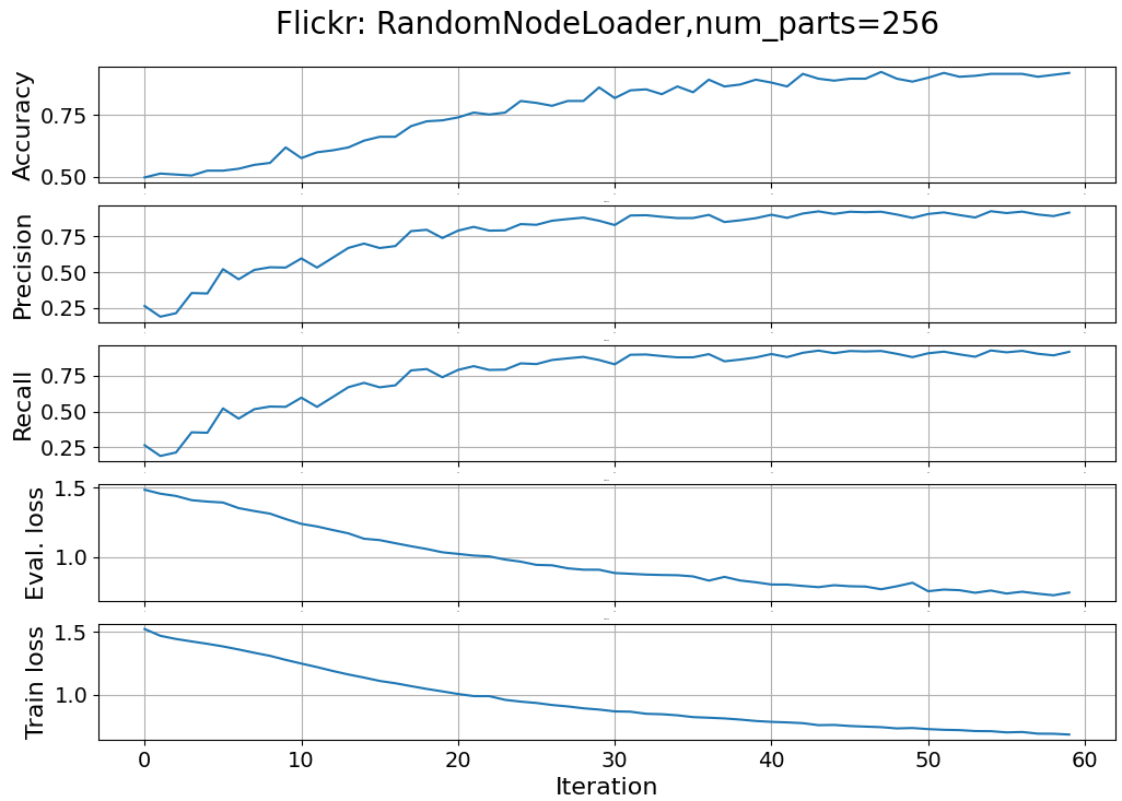
Fig 6. Performance metrics and loss for a GCN in a multi-label classification of data loaded randomly
Neighbor Node Loader
The configuration parameters used for this loader include:
- num_neighbors: Specifies the number of neighbors to sample at each layer or hop in a Graph Neural Network. It is defined as an array, e.g., `[num_neighbors_first_hop, num_neighbors_second_hop, ...]`.
- replace: Determines whether sampling is performed with or without replacement.
- batch_size; Size of the batch
We specify few other parameters which value do not vary during our evaluation>
- drop_last: to drop the last batch is it is less that the prescribed batch_size
- input_nodes for the applying the mask for training and validation data
# --- Code Snippet 4 ---
     def __neighbors_loader(self) -> (DataLoader, DataLoader):
     # Extract loader configuration
   num_neighbors = self.attributes_map['num_neighbors']
   batch_size = self.attributes_map['batch_size']
   replace = self.attributes_map['replace']

    # Generate the loader for training data
    train_loader = NeighborLoader(self.data,
                                                     num_neighbors=num_neighbors,
                                                     batch_size=batch_size,
                                                     replace=replace,
                                                     drop_last=False,
                                                     shuffle=True,
                                                     input_nodes=self.data.train_mask)

        # Generate the loader for validation data
    val_loader = NeighborLoader(self.data,
                                                   num_neighbors=num_neighbors,
                                                   batch_size=batch_size,
                                                   replace=replace,
                                                   drop_last=False,
                                                   shuffle=False,
                                                   input_nodes=self.data.val_mask)
return train_loader, val_loader
We only need to update the dictionary of this loader configuration parameters in the code snippet 3.
# --- Code Snippet 5 ---
    attrs = {
      'id': 'NeighborLoader',
      'num_neighbors': [6, 4],
      'batch_size': 1024,
      'replace': True
}
The training and validation of the Graph Convolutional Neural Network produces the following plots for the performance metrics and losses.

Fig 7. Performance metrics and loss for a GCN in a multi-label classification of data loaded with a Neighbor loader
Graph Sampling Based Inductive Learning loader
For evaluating this loader, we use the following configuration parameters:
- walk_length: Defines the number of hops (nodes) in a single random walk
- batch_size: Size of the batch of subgraph
- num_steps: Number of times new nodes are samples in each epoch
- sample_coverage: Number of times each node is sampled: appeared in a batch.
                          # --- Code Snippet 6 ---

def __graph_saint_random_walk(self,
                                                          num_workers: int) -> (DataLoader, DataLoader):

        # Dynamic configuration parameter for the loader
     walk_length = self.attributes_map['walk_length']
     batch_size = self.attributes_map['batch_size']
     num_steps = self.attributes_map['num_steps']
     sample_coverage = self.attributes_map['sample_coverage']

        # Extraction of the loader for training data
     train_loader = GraphSAINTRandomWalkSampler(data=self.data,
                                                   batch_size=batch_size,
                                                   walk_length=walk_length,
                                                   num_steps=num_steps,
                                                   sample_coverage=sample_coverage,
                                                   shuffle=True)

        # Extraction of the loader for validation data
     val_loader = GraphSAINTRandomWalkSampler(data=self.data,
                                                 batch_size=batch_size,
                                                 walk_length=walk_length,
                                                 num_steps=num_steps,
                                                 sample_coverage=sample_coverage,
                                                 shuffle=False)
   return train_loader, val_loader
Once again, we reuse the implementation in code snippet 3 and update the dictionary of this loader configuration parameters.
                        # --- Code Snippet 7 ---

attrs = {
     'id': 'GraphSAINTRandomWalkSampler',
'walk_length': 3,
'num_steps': 12,
'sample_coverage': 100,
'batch_size': 4096
}

Fig 8. Performance metrics and loss for a GCN in a multi-label classification of data loaded with a Graph SAINT random walk loader
The performance metrics, accuracy, precision and recall points to an inability for the Random walk to capture long-range dependencies.
Comparison
Lastly, let's compare the impact of each data loader on the precision of the graph convolutional neural network..

Fig 9. Plotting precision in a multi-label classification of a GCN with various graph data loaders
Although the random walk for the GraphSAINTRandomWalk loader excels in analyzing and representing local structure, it fails to capture the global context (high number of hops - dependencies) of a large image set. Moreover, the plot highlights the high degree of instability of performance metrics even though the loss in the validation run converges appropriately.
NeighborNodeLoader select nodes across multiple hops and therefore avoid over emphasis on nodes sampled in nearby regions.
Here is a summary of benefits, drawbacks and applicability of the 3 graph data loaders.

Table 2. Pros and cons of Random node, Neighbor node and Random walk loaders

