Showing posts with label Gradient. Show all posts

Wednesday, April 3, 2024

Geometric Learning in Python: Vector Operators

Target audience: Beginner
Estimated reading time: 5'
Physics-Informed Neural Networks (PINNs) are gaining popularity for integrating physical laws into deep learning models. Essential tools like vector operators, including the gradient, divergence, curl, and Laplacian, are crucial in applying these constraints.


Table of contents

Follow me on LinkedIn

What you will learn: How to implement the vector gradient, divergence, curl and laplacian operators in Python using SymPy library.

Notes
  • Environments: Python  3.10.10,  SymPy 1.12, Matplotlib 3.8.2
  • This article assumes that the reader is familiar with differential and tensor calculus.
  • Source code is available at github.com/patnicolas/Data_Exploration/diffgeometry
  • To enhance the readability of the algorithm implementations, we have omitted non-essential code elements like error checking, comments, exceptions, validation of class and method arguments, scoping qualifiers, and import statements.

Introduction

Geometric learning addresses the difficulties of limited data, high-dimensional spaces, and the need for independent representations in the development of sophisticated machine learning models.

Note: This article is the 5th installment in our series on Geometric Learning in Python following
The following description of vector differential operators leverages some of concept defined in the previous articles in the Geometric Learning in Python series and SymPy library.

SymPy is a Python library dedicated to symbolic mathematics. Its implementation is as simple as possible to be comprehensible and easily extensible with support for differential and integral calculus, Matrix operations, algebraic and polynomial equations, differential geometry, probability distributions, 3D plotting. The source code is available at  github.com/sympy/sympy.git

In tensor calculus, a vector operator is a type of differential operator:
  • The gradient transforms a scalar field into a vector field.
  • The divergence changes a vector field into a scalar field.
  • The curl converts a vector field into another vector field.
  • The laplacian takes a scalar field and yields another scalar field.

Gradient

Consider a scalar field f in a 3-dimension space. The gradient of this field is defined as the vector of the 3 partial derivatives with respect to xy and z [ref 1].\[\triangledown f= \frac{\partial f}{\partial x} \vec{i} + \frac{\partial f}{\partial y} \vec{j} + \frac{\partial f}{\partial z} \vec{k}\]
We create a class, VectorOperators, that wraps the following operators:  gradient, divergence, curl and laplacian. The constructor initializes the function as an expression for which the various operators are applied to.

class VectorOperators(object):
    def __init__(self, expr: Expr):     # Expression for the input function
        self.expr = expr

    def gradient(self) -> VectorZero:
        from sympy.vector import gradient

        return gradient(self.expr, doit=True)

Let's calculate the gradient vector for the function \[f(x,y,z)=x^{2}+y^{2}+z^{2} \] , as depicted in the plot below.

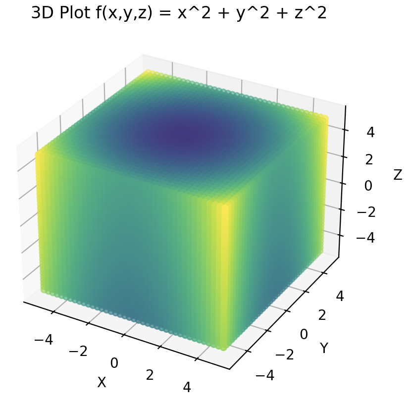
Fig. 1  3D visualization of function f(x,y,z) = x**2 + y**2 + z**2

The Python for the visualization of the function is described in Appendix (Visualization function)

The following code snippet computes the gradient of this function as \[\triangledown f(x,y,z) = 2x.\vec{i} + 2y.\vec{j} + 2y.\vec{k}\] 
r = CoordSys3D('r')
f = r.x*r.x+r.y*r.y+r.z*r.z

vector_operator = VectorOperators(f)
grad_f = vector_operator.gradient()    # 2*r.x + 2*r.y+ 2*r.z

The function f is defined using the default Euclidean coordinates rThe gradient is depicted in the following plot implemented using Matplotlib module. The actual implementation is described in Appendix (Visualization gradient)

Fig. 2  3D visualization of grad_f(x,y,z) = 2x.i + 2y.j + 2z.k


Divergence

Divergence is a vector operator used to quantify the strength of a vector field's source or sink at a specific point, producing a signed scalar value. When applied to a vector F, comprising components XY, and Z, the divergence operator consistently yields a scalar result [ref 2]\[div(F)=\triangledown .F=\frac{\partial X}{\partial x}+\frac{\partial Y}{\partial y}+\frac{\partial Z}{\partial z}\]
Let's implement the computation of the divergence as method of the class VectorOperators:

def divergence(self, base_vec: Expr) -> VectorZero:
    from sympy.vector import divergence

    div_vec = self.expr*base_vec
    return divergence(div_vec, doit=True)

Using the same instance vector_operators as with the gradient calculation:
divergence = vector_operators.divergence(r.i + r.j + r.k)

The execution of the code above produces the following:\[div(f(x,y,z)[\vec{i} + \vec{j}+ \vec{k}]) = 2x(y+z+xy)\]


Curl

In mathematics, the curl operator represents the minute rotational movement of a vector in three-dimensional space. This rotation's direction follows the right-hand rule (aligned with the axis of rotation), while its magnitude is defined by the extent of the rotation [ref 2]. Within a 3D Cartesian system, for a three-dimensional vector F, the curl operator is defined as follows: \[ \triangledown * \mathbf{F}=\left (\frac{\partial F_{z}}{\partial y}- \frac{\partial F_{y}}{\partial z} \right ).\vec{i} + \left (\frac{\partial F_{x}}{\partial z}- \frac{\partial F_{z}}{\partial x} \right ).\vec{j} + \left (\frac{\partial F_{y}}{\partial x}- \frac{\partial F_{x}}{\partial y} \right ).\vec{k} \]. Let's add the curl method to our class VectorOperator as follow:

def curl(self, base_vectors: Expr) -> VectorZero:
    from sympy.vector import curl

    curl_vec = self.expr*base_vectors
    return curl(curl_vec, doit=True)

For the sake of simplicity let's compute the curl along the two base vectors j and k:
curl_f = vector_operator.curl(r.j+r.k)    # j and k direction only

The execution of the curl method outputs: \[curl(f(x,y,z)[\vec{j} + \vec{k}]) = x^{2}\left ( z-y \right).\vec{i}-2xyz.\vec{j}+2xyz.\vec{k}\]


Laplacian

In mathematics, the Laplacian, or Laplace operator, is a differential operator derived from the divergence of the gradient of a scalar function in Euclidean space [ref 3].  The Laplacian is utilized in various fields, including calculating gravitational potentials, solving heat and wave equations, and processing images.
It is a second-order differential operator in n-dimensional Euclidean space and is defined as follows: \[\triangle f= \triangledown ^{2}f=\sum_{i=1}^{n}\frac{\partial^2 f}{\partial x_{i}^2}\]. The implementation of the method laplacian reflects the operator is the divergence (step 2) of the gradient (Step 1)

def laplacian(self) -> VectorZero:
   from sympy.vector import divergence, gradient
        
   # Step 1 Compute the Gradient vector
   grad_f = self.gradient()
        
   # Step 2 Apply the divergence to the gradient
   return divergence(grad_f)

Once again we leverage the 3D coordinate system defined in SymPy to specify the two functions for which the laplacian has to be evaluated

r = CoordSys3D('r')
    
f = r.x*r.x + r.y*r.y + r.z*r.z
vector_operators = VectorOperators(f)
laplace_op = vector_operators.laplacian()
print(laplace_op)       # 6

f = r.x*r.x*r.y*r.y*r.z*r.z  
vector_operators = VectorOperators(f)
laplace_op = vector_operators.laplacian()
print(laplace_op)     # 2*r.x**2*r.y**2 + 2*r.x**2*r.z**2 + 2*r.y**2*r.z**2

Outputs: \[\triangle (x^{2} + y^{2}+z^{2}) = 6\] \[\triangle (x^{2}y^{2}z^{2})=2(x^{2}y^2 +x^{2}z^{2}+y^{2}z^{2}) \]


-------------
Patrick Nicolas has over 25 years of experience in software and data engineering, architecture design and end-to-end deployment and support with extensive knowledge in machine learning. 
He has been director of data engineering at Aideo Technologies since 2017 and he is the author of "Scala for Machine Learning", Packt Publishing ISBN 978-1-78712-238-3

Appendix

Visualization function

The implementation relies on 
  • Numpy meshgrid to setup the axis and values for the x, y and z axes. 
  • Matplotlib scatter method to display the values generated by the function f
The function to plot takes x, y and z grid values and to generate data f(x,y,z)

@staticmethod
def show_3D_function(f: Callable[[float, float, float], float], grid_values: np.array) -> NoReturn:
   import matplotlib.pyplot as plt
   from mpl_toolkits.mplot3d import axes3d

        # Setup the grid with the appropriate units and boundary
   x, y, z = np.meshgrid(grid_values, grid_values, grid_values)

        # Apply the function f
   data = f(x, y, z)

        # Set up plot (labels, legend,..)
   ax: Axes =  self.__setup_3D_plot('3D Plot f(x,y,z) = x^2 + y^2 + z^2')
        
        # Display the data along x, y and z using scatter plot
   ax.scatter(x, y, z, c=data) 
   plt.show()


Visualization gradient

The 3 components of the gradient vector as passed as argument, grad_f.
The implementation relies on 
  • Numpy meshgrid to setup the axis and values for the x, y and z axes. 
  • Matplotlib quiver method to display the gradient vectors at each grid values  
@staticmethod
def show_3D_gradient(grad_f: List[Callable[[float], float]], grid_values: np.array) -> NoReturn:
    import matplotlib.pyplot as plt
    from mpl_toolkits.mplot3d import axes3d

        # Setup the grid with the appropriate units and boundary
    x, y, z = np.meshgrid(grid_values, grid_values, grid_values)
    ax = self.__setup_3D_plot('3D Plot Gradient 2x.i + 2y.j + 2z.k')

        # Extract the gradient df/dx, df/dy and df/dz
    X = grad_f[0](x)
    Y = grad_f[1](y)
    Z = grad_f[2](z)

        # Display the gradient vectors as vector fields
    ax.quiver(x, y, z, X, Y, Z, length=1.5, color='grey', normalize=True)
    plt.show()


Thursday, March 14, 2024

Geometric Learning in Python: Differential Operators

Target audience: Intermediate
Estimated reading time: 5'

The use of Riemannian manifolds and topological computing is gaining traction in machine learning circles as a means to surpass the existing constraints of data analysis within Euclidean space. 
This article aims to present the fundamental aspects of differential geometry.


Table of content
      Why SymPy
      Gradient
      Divergence
      Curl
      Validation
      Laplace
      Fourier
Follow me on LinkedIn

What you will learn: Vector fields, Differential operators and integral transforms as key components of differential geometry applied to deep learning.

Notes
  • Environments: Python  3.10.10 and SymPy 1.12
  • The differential operators are used in a future post dedicated to differential geometry and manifold learning
  • This article assumes that the reader is familiar with differential calculus and basic concept of geometry
  • Source code is available at github.com/patnicolas/Data_Exploration/diffgeometry
  • To enhance the readability of the algorithm implementations, we have omitted non-essential code elements like error checking, comments, exceptions, validation of class and method arguments, scoping qualifiers, and import statements.

Overview

The heavy dependence on elements from Euclidean space for data analysis and pattern recognition in machine learning might be approaching a threshold. Incorporating differential geometry and Riemannian manifolds has already shown beneficial effects on the accuracy of deep learning models, as well as on reducing their development costs [ref 1].

Why differential geometry

Conventional approaches in machine learning, pattern recognition, and data analysis often presuppose that input data can be effectively represented using elements from Euclidean space. Although this assumption has been sufficient for numerous applications in the past, there's a growing awareness among data scientists and engineers that most data in vision and pattern recognition actually reside in a differential manifold (feature space) that's embedded within the raw data's Euclidean space
Leveraging this geometric information can result in a more precise representation of the data's inherent structure, leading to improved algorithms and enhanced performance in real-world applications [ref 2].

Why SymPy

SymPy is a Python library dedicated to symbolic mathematics. Its implementation is as simple as possible in order to be comprehensible and easily extensible. It is licensed under BSD. SymPy supports differential and integral calculus, Matrix operations, algebraic and polynomial equations, differential geometry, probability distributions, 3D plotting and discrete math [ref 3].
To install pip install sympy
Source code for SymPy is available at github.com/sympy/sympy.git

This article has 3 sections:
  1. Introduction of vector fields and implementation in SymPy
  2. Differential operators (Gradient, Divergence and Curl)
  3. Laplace and Fourier Transform

Vector fields

Let's start with an overview of vector fields as the basis of differential geometry [ref 4].
Consider a three-dimensional Euclidean space characterized by basis vectors {ei} and a vector field V, expressed as (f1, f2, f3). In this scenario, it is crucial to note that we are following the conventions of Einstein's tensor notation.

Visualization of a vector field in 3D Euclidean space

The vector field at the point P(x,y,z) is defined as the tuple (f1(x,y,z), f2(x,y,z), f3(x,y,z)). The vector over a field of n dimension field and basis vectors  {ei}  can be formally defined as \[f: \boldsymbol{x} \,\, \epsilon \,\,\, \mathbb{R}^{n} \mapsto \mathbb{R} \\ f(\mathbf{x})=\sum_{i=1}^{n}{f^{i}}(\mathbf{x}).\mathbf{e}_{i}\] Example for 3 dimension space: \[f(x,y,z) = (2x+z^{3})\boldsymbol{\mathbf{\overrightarrow{i}}} + (xy+e^{-y}-z^{2})\boldsymbol{\mathbf{\overrightarrow{j}}} + \frac{x^{3}}{y}\boldsymbol{\mathbf{\overrightarrow{k}}}\] Let's carry out the creation of this vector field, f, in SymPy and compute its value at f(1.0, 2.0, 0.5). To begin, we need to establish a 3D coordinate system, denoted as r, and then express the vector using r.

from sympy.vector import CoordSys3D
from sympy import exp
r = CoordSys3D('r') f = (2*r.x + r.z**3)*r.i + (r.x*r.y+sympy.exp(-r.y)-r.z**2)*r.j + (r.x**3/r.y)*r.k

w = f.evalf(subs={r.x: 1.0, r.y: 2.0, r.z: 0.2})
print(w)                                 # 2.008*r.i + 2.09533528323661*r.j + 0.5*r.k

Now, let's consider the same vector V with a second reference; origin 0' and basis vector e'i
Visualization of two coordinate systems

\[f(\mathbf{x})=\sum_{i=1}^{n} f'^{i}(\mathbf{x}).\mathbf{e'}_{i}\] The transformation matrix Sij convert the coordinates value functions  fi and f'i. The tuple f =(fiis the co-vector field for the vector field V 
\[S_{ij}: \begin{Vmatrix} f^{1} \\ f^{2} \\ f^{3} \end{Vmatrix} \mapsto \begin{Vmatrix} f'^{1} \\ f'^{2} \\ f'^{3} \end{Vmatrix}\] The scalar product of the co-vector f' and vector v(f) is defined as \[< f',v> = \sum f'_{i}.f^{i}\] Given the scalar product we can define the co-vector field f' as a linear map \[\alpha (v) = < f',v> (1) \] 

Differential operators

Let's demonstrate how to calculate differential operators using the SymPy library within a 3D Cartesian coordinate system. To begin, we'll create a class named DiffOperators which will encapsulate the implementation of various differential operators and transforms.

Gradient

Consider a scalar field f in a 3-dimension space. The gradient of this field is defined as the vector of the 3 partial derivatives f with respect to x, y and z [ref 5].\[\triangledown f= \frac{\partial f}{\partial x} \vec{i} + \frac{\partial f}{\partial y} \vec{j} + \frac{\partial f}{\partial z} \vec{k}\]

class DiffOperators(object):
    def __init__(self, expr: Expr):
        self.expr = expr

    def gradient(self) -> VectorZero:
        from sympy.vector import gradient

        return gradient(self.expr, doit=True)
Example of input function: \[f(x,y,z)=x^{2}yz\]
r = CoordSys3D('r')
this_expr = r.x*r.x*r.y*r.z

diff_operator = DiffOperators(this_expr)
grad_res = diff_operator.gradient()
\[\triangledown f(x,y,z) = 2xyz.\vec{i} + x^{2}z.\vec{j} + x^{2}y.\vec{k}\]

Divergence

Divergence is a vector operator used to quantify the strength of a vector field's source or sink at a specific point, producing a signed scalar value. When applied to a vector F, comprising components X, Y, and Z, the divergence operator consistently yields a scalar result [ref 6].
\[div(F)=\triangledown .F=\frac{\partial X}{\partial x}+\frac{\partial Y}{\partial y}+\frac{\partial Z}{\partial z}\]
def divergence(self, base_vec: Expr) -> VectorZero:
    from sympy.vector import divergence

    div_vec = self.expr*base_vec
    return divergence(div_vec, doit=True)
Using the same input expression as used for the gradient calculation:
div_res = diff_operator.divergence(r.i + r.j + r.k)
\[div(f(x,y,z)[\vec{i} + \vec{j}+ \vec{k}]) = 2x(y+z+xy)\]

Curl

In mathematics, the curl operator represents the minute rotational movement of a vector in three-dimensional space. This rotation's direction follows the right-hand rule (aligned with the axis of rotation), while its magnitude is defined by the extent of the rotation [ref 6]. Within a 3D Cartesian system, for a three-dimensional vector F, the curl operator is defined as follows:
\[ \triangledown * \mathbf{F}=\left (\frac{\partial F_{z}}{\partial y}- \frac{\partial F_{y}}{\partial z} \right ).\vec{i} + \left (\frac{\partial F_{x}}{\partial z}- \frac{\partial F_{z}}{\partial x} \right ).\vec{j} + \left (\frac{\partial F_{y}}{\partial x}- \frac{\partial F_{x}}{\partial y} \right ).\vec{k} \]
def curl(self, base_vectors: Expr) -> VectorZero:
    from sympy.vector import curl

    curl_vec = self.expr*base_vectors
    return curl(curl_vec, doit=True)

If we use only the two base vectors j and k:
curl_res = diff_operator.curl(r.j+r.k)
\[curl(f(x,y,z)[\vec{j} + \vec{k}]) = x^{2}\left ( z-y \right ).\vec{i}-2xyz.\vec{i}+2xyz.\vec{k}\]

Validation

We can confirm the accuracy of the gradient, divergence, and curl operators implemented in SymPy by utilizing the subsequent formulas:  \[curl(\triangledown f))= \triangledown *\left ( \triangledown f\right ) = 0\]  and  \[\triangledown . curl (F) = \triangledown .\left ( \triangledown * F \right ) = 0\]
grad_res = diff_operator.gradient()
assert(diff_operator.curl(grad_res) ==0)   # Print 0

curl_res = diff_operator.curl(r.i + r.j + r.k)
assert(diff_operator.divergence(curl_res) == 0) # Print 0


Transforms

An integral transform transforms a function from the time domain into its equivalent representation in the frequency domain, as depicted in the following diagram:

Illustration of conversion from time domain to frequency domains

The evaluation of SymPy functions follows a two-step process:
  1. Generate function F in frequency space
  2. Evaluate output of F for given input values.

Laplace

The Laplace transform is a type of integral transform that changes a function of a real variable (typically time, t) into a function in the s-plane, which is a variable in the complex frequency domain [ref 7].. Specifically, it transforms ordinary differential equations into algebraic ones and converts convolution operations into simpler multiplication. The formulation of the Laplace transform is:\[\mathfrak{L}[f(t)](s)=\int_{0}^{+\inf}f(t).e^{-st}dt\]
def laplace(self):
    from sympy import laplace_transform
        
    return laplace_transform(self.expr, t, s, noconds=True)


Let's create the Laplace transforms for two basic functions and then calculate the outcomes of these transformed functions in the frequency domain, using the values s=0.5 and a=0.2.
t, s = sympy.symbols('t, s', real=True)
a = sympy.symbols('a', real=True)
diff_operator = DiffOperators(sympy.exp(-a*t))
laplace_func = diff_operator.laplace()

print(Laplace_func.evalf(subs={s:0.5, a:0.2}))   #  1.4285
\[\int_{0}^{+\inf}e^{-at}.e^{-st}dt = \frac{1}{a+s}\]
diff_operator = DiffOperators(sympy.sqrt(-a*t))
laplace_func = diff_operator.laplace() 

print(Laplace_func.evalf(subs={s:0.5, a:0.2}))   #  1.1209
\[\int_{0}^{+\inf}\sqrt{at}.e^{-st}dt = \frac{\sqrt{a\pi}}{2.s^{3/2}}\]

Fourier

Like the Laplace transform, the Fourier transform is another integral transform that translates a function into a version that represents the frequencies contained in the original function. The result of this transformation is a complex-valued function dependent on frequency [ref 8]. Often referred to as the frequency domain representation of the original function, the formulation of the Fourier transform is as follows: \[F(x )=\int_{-\inf}^{+\inf}f(t).e^{-2\pi itx}dt\] The implementation uses the SymPy function fourier_transform which takes the function (self.expr) and x, and k parameters as arguments.
def fourier(self):
   from sympy import fourier_transform
     
   return fourier_transform(self.expr, x, k)

Let's implement the Fourier transforms for two simple functions, exp and sin, and then calculate the outcomes of these transformed functions in the frequency domain with k=0.4
x, k = sympy.symbols('x, k', real=True)
diff_operator = DiffOperators(sympy.exp(-x**2))

fourier_func = diff_operator.fourier()
print(fourier_func.evalf(subs={k: 0.4}))       # 0.3654
\[\int_{-\inf}^{+\inf}e^{-t^{2}}.e^{-2\pi itx}dt = \sqrt{\pi}.e^{-2\pi x^{2}}\]
diff_operator = DiffOperators(sympy.sin(x))
diff_operator.fourier()
\[\int_{-\inf}^{+\inf}\sin(t).e^{-2\pi itx}dt = 0\]


Thank you for reading this article. For more information ...

References


---------------------------
Patrick Nicolas has over 25 years of experience in software and data engineering, architecture design and end-to-end deployment and support with extensive knowledge in machine learning. 
He has been director of data engineering at Aideo Technologies since 2017 and he is the author of "Scala for Machine Learning" Packt Publishing ISBN 978-1-78712-238-3