Geometric Learning in Python: Vector & Covector Fields

Target audience: Beginner

Estimated reading time: 5'

Posts history

The use of Riemannian manifolds and topological computing is gaining traction in machine learning circles to surpass the existing constraints of data analysis within Euclidean space. 

This article aims to present one of the fundamental aspects of differential geometry: vector and covector fields.

Table of contents

Introduction

        Differential geometry

        SymPy library

Vector vs. vector field

Vector fields

        Overview

        Implementation

Covector fields

References

What you will learn: Vector and covector fields in differential geometry applied to machine learning with implementation in 2D and 3D dimensional use cases.

Notes: 

• Environments: Python  3.10.10 and SymPy 1.12
• This article assumes that the reader is familiar with differential calculus and basic concept of geometry.
• Source code is available at github.com/patnicolas/Data_Exploration/diffgeometry
• To enhance the readability of the algorithm implementations, we have omitted non-essential code elements like error checking, comments, exceptions, validation of class and method arguments, scoping qualifiers, and import statements.

Introduction

The heavy dependence on elements from Euclidean space for data analysis and pattern recognition in machine learning might be approaching a threshold. Incorporating differential geometry and Riemannian manifolds has already shown beneficial effects on the accuracy of deep learning models, as well as on reducing their development costs [ref 1]. 

This article is the 4th installment in our series on Geometric Learning in Python following

• Geometric Learning in Python: Basics introduces differential geometry as an applied to machine learning and its basic components.
• Geometric Learning in Python: Manifolds describes manifold components such as tangent vectors, geodesics with implementation in Python for Hypersphere using the Geomstats library.
• Geometric Learning in Python: Intrinsic Representation Reviews the various coordinates system using extrinsic and intrinsic representation.
  

Differential geometry

Conventional approaches in machine learning, pattern recognition, and data analysis often presuppose that input data can be effectively represented using elements from Euclidean space. Although this assumption has been sufficient for numerous applications in the past, there's a growing awareness among data scientists and engineers that most data in vision and pattern recognition reside in a differential manifold (feature space) that's embedded within the raw data's Euclidean space. 
Leveraging this geometric information can result in a more precise representation of the data's inherent structure, leading to improved algorithms and enhanced performance in real-world applications [ref 2].

 

SymPy library

SymPy is a Python library dedicated to symbolic mathematics. Its implementation is as simple as possible to be comprehensible and easily extensible. It is licensed under BSD. SymPy supports differential and integral calculus, Matrix operations, algebraic and polynomial equations, differential geometry, probability distributions, 3D plotting and discrete math [ref 3].

• To install pip install sympy
• Source code for SymPy is available at github.com/sympy/sympy.git

Vector vs. vector field

A vector and a vector field are both involving vectors, but they have different meanings:

• Vector: A vector is a mathematical object that represents a quantity with both magnitude and direction. In physics and geometry, vectors are often represented by arrows, where the length of the arrow corresponds to the magnitude of the vector and the direction of the arrow indicates the direction of the vector. Vectors can exist in various dimensions (such as 2D, 3D, or higher dimensions)
• Vector Field: A vector field is a function that assigns a vector to each point in each space. In other words, at every point in the space, there is a corresponding vector. Vector fields are used to describe various physical phenomena where vector quantities vary continuously across space. 

 

Vector fields

Overview

In tensor calculus, a vector field refers to the assignment of a vector to every point within a space, typically within Euclidean space. Visualizing a vector field on a plane involves picturing a series of arrows, each representing a vector with specific magnitudes and directions, anchored at individual points across the plane.

Fig 1 Visualization of vector fields on a sphere in 3D space

Let's start with an overview of vector fields as the basis of differential geometry [ref 4]. Consider a three-dimensional Euclidean space characterized by basis vectors {eⁱ} and a vector field V, expressed as  {fⁱ}  =(f, f2, f3 )  . 

Fig. 2 Visualization of a vector field in 3D Euclidean space

The vector field at the point P(x,y,z) is defined as the tuple (f₁(x,y,z), f₂(x,y,z), f₃(x,y,z)). The vector over a field of n dimension field and basis vectors  {eⁱ}  can be formally defined as: \[f: \boldsymbol{x} \,\, \epsilon \,\,\, \mathbb{V} \mapsto \mathbb{R}^{n} \\ f(\mathbf{x})=\sum_{i=1}^{n}{f^{i}}(\mathbf{x}).\mathbf{e}_{i} \ \ \ e_{i}=\frac{\partial }{\partial x^{i}}\]

Implementation

Example for 2 dimension space: \[f(x,y)=\frac{-y}{\sqrt{x^{2}+y^{2}}} \vec{i} + \frac{x}{\sqrt{x^{2}+y^{2}}} \vec{j} \ \ \ (1) \] Let's carry out the creation of this vector field, f defined in the formula (1) in SymPy and compute its value at f(1.0, 2.0). To begin, we need to establish a 2D coordinate system, denoted as cs, and then express the vector field as the sum of the two base scalar field f1 and f2.

import sympy
import math
from sympy import symbols
from sympy.diffgeom import Manifold, Patch, CoordSystem, BaseScalarField

x, y = symbols('x, y', real=True)
cs= CoordSystem('x y', Patch('P', Manifold('square', 2)))

norm = sympy.sqrt(x*x + y+y)
f1 = BaseScalarField(cs, 0)
f2 = BaseScalarField(cs, 1)
f = -f2/norm + f1/norm
w = f.evalf(subs={x: 1.0, y: 2.0})
print(w)

The visualization of this 2-dimension field is as follow:

• Set up the mesh grid
• Implement the vector field f
• Display the vector field using the quiver method from Matplotlib module.

import matplotlib.pyplot as plt
import numpy as np

# Set up the mesh grid
grid_values = np.linspace(-8, 8, 16)
n_x, n_y = np.meshgrid(grid_values, grid_values)

# Define the vector field
np_norm = np.sqrt(n_x**2 + n_y**2)
X = -n_y/np_norm
Y = n_x/np_norm

# Display
plt.quiver(n_x, n_y, X, Y, color='red')
plt.show()

Fig. 3 Visualization of a vector field f(x,y) defined in formula (1)

Example for 3 dimension space: \[f(x,y,z) = (2x+z^{3})\boldsymbol{\mathbf{\overrightarrow{i}}} + (xy+e^{-y}-z^{2})\boldsymbol{\mathbf{\overrightarrow{j}}} + \frac{x^{3}}{y}\boldsymbol{\mathbf{\overrightarrow{k}}} \ \ \ (2) \]  Let's carry out the creation of this vector field, f, in SymPy and compute its value at f(1.0, 2.0, 0.5). To begin, we need to establish a 3D coordinate system, denoted as r, and then express the vector using r.

Note: Contrary to the example with a 2-dimension field which require to define explicitly the coordinate system, this 3D vector field leverage an existing 3D coordinate, CoordSys3D

from sympy.vector import CoordSys3D
from sympy import exp

r = CoordSys3D('r')

f = (2 * r.x + r.z ** 3) * r.i + (r.x * r.y + sympy.exp(-r.y) - r.z ** 2) * r.j + (r.x ** 3 / r.y) * r.k
w = f.evalf(subs={r.x: 1.0, r.y: 2.0, r.z: 0.2})    # 2.008*r.i + 2.09533528323661*r.j + 0.5*r.k

print(w)

The visualization of the 3-dimension vector field (2) is very similar to the visualization of the 2-dimension field (1).

# Set up a 8 x8 x8  mesh grid
grid_values = np.linspace(0.1, 0.9, 8)
n_x, n_y, n_z = np.meshgrid(grid_values, grid_values, grid_values)

# Implement the 3 components of vector field
#. f = Xi + yJ + Zj
X = 2*n_x+n_z**3
Y = n_x*n_y + np.exp(-n_y) - n_z**2
Z = n_x**3/n_y

# Display the vector field in 3D
fig = plt.figure()
ax = fig.add_subplot(projection='3d')
ax.quiver(n_x, n_y, n_z, X, Y, Z, length=0.2, color='blue', normalize=True)
plt.show()

Fig. 4 Visualization of a vector field f(x, y, z) defined in formula (2)

Covector fields

Covariant vectors (or tensors) are fundamental concepts in the field of tensor calculus and differential geometry, used to describe geometric and physical entities in a way that is independent of the coordinate system used. \[df: V\rightarrow \mathbb{R}\]

\[f^*: f\rightarrow  df=\sum_{i=1}^{n}\frac{\partial f}{\partial x^{i}}dx_{i}\] For a co-vector field (or differential form) along a vector v: \[df(\vec{v})=\triangledown f.\vec{v}\]

Let's consider a very simple vector field: \[f(x, y)=x\vec{i} + y\vec{j} \ \ \ (3) \] and co-vector field: \[dx=\frac{1}{n} \ \ dy=\frac{1}{n} \ \ \ n=1,\infty\]

The following code snippet illustrates the vector field and co-vector field for (3).

# Limit values for vector and covector fields
_min = -8
_max = 8

fig, ax = plt.subplots()

# Generate co-vector fields
co_vectors = [{'center': (0.0, 0.0), 'radius': _max*(1.0 - 1.0/n), 'color': 'blue', 'fill': False}
       for n in range(1, 10)]

[plt.gca().add_patch(Circle(circle['center'], circle['radius'], color=circle['color'], fill=circle['fill']))
       for circle in co_vectors]

# Set limits for x and y axes
ax.set_aspect('equal')
ax.set_xlim(_min, _max)
ax.set_ylim(_min, _max)
        
# Set up the grid
grid_values = np.linspace(_min, _max, _max-_min)
x, y = np.meshgrid(grid_values, grid_values)
        
# Display vector and co-vector fields
plt.quiver(x, y, x, y, color='red')
plt.show()

The vector field is represented by red arrows while the co-vector fields is represented by the blue circle (levels set).

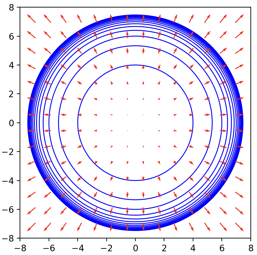
Fig. 5 Visualization of a vector field and co-vector field for f(x, y) = (x, y) 

As depicted in the plot above, vector fields exhibit contravariant behavior, meaning that the field's intensity (represented by arrow size) amplifies as we move away from the origin. Conversely, covector fields demonstrate covariant behavior, resulting in a decrease in the spacing between the field's level sets as we move away from the origin.

References

[1] Introduction to Tensors - Universität des Saarlandes, Saarbrücken

[2] YouTube: Tensor Calculus Series - Eigenchris

[3] Vector and Tensor Analysis with Applications -  A. I. Borisenko, I. E. Tarapov - Dover Books on MathenaticsPublications 1979 

[4] A Student's Guide to Vectors and Tensors - D. Fleisch - Cambridge University Press - 2008

-------------
Patrick Nicolas has over 25 years of experience in software and data engineering, architecture design and end-to-end deployment and support with extensive knowledge in machine learning. 
He has been director of data engineering at Aideo Technologies since 2017 and he is the author of "Scala for Machine Learning", Packt Publishing ISBN 978-1-78712-238-3