
Target audience: Intermediate
Estimated reading time: 5'
The use of Riemannian manifolds and topological computing is gaining traction in machine learning circles as a means to surpass the existing constraints of data analysis within Euclidean space.
This article aims to present the fundamental aspects of differential geometry.

What you will learn: Vector fields, Differential operators and integral transforms as key components of differential geometry applied to deep learning.
Notes:
- Environments: Python 3.10.10 and SymPy 1.12
- The differential operators are used in a future post dedicated to differential geometry and manifold learning
- This article assumes that the reader is familiar with differential calculus and basic concept of geometry
- Source code is available at github.com/patnicolas/Data_Exploration/diffgeometry
- To enhance the readability of the algorithm implementations, we have omitted non-essential code elements like error checking, comments, exceptions, validation of class and method arguments, scoping qualifiers, and import statements.
Overview
The heavy dependence on elements from Euclidean space for data analysis and pattern recognition in machine learning might be approaching a threshold. Incorporating differential geometry and Riemannian manifolds has already shown beneficial effects on the accuracy of deep learning models, as well as on reducing their development costs [ref 1].
Why differential geometry
Conventional approaches in machine learning, pattern recognition, and data analysis often presuppose that input data can be effectively represented using elements from Euclidean space. Although this assumption has been sufficient for numerous applications in the past, there's a growing awareness among data scientists and engineers that most data in vision and pattern recognition actually reside in a differential manifold (feature space) that's embedded within the raw data's Euclidean space.
Leveraging this geometric information can result in a more precise representation of the data's inherent structure, leading to improved algorithms and enhanced performance in real-world applications [ref 2].
Why SymPy
SymPy is a Python library dedicated to symbolic mathematics. Its implementation is as simple as possible in order to be comprehensible and easily extensible. It is licensed under BSD. SymPy supports differential and integral calculus, Matrix operations, algebraic and polynomial equations, differential geometry, probability distributions, 3D plotting and discrete math [ref 3].
To install pip install sympy
Source code for SymPy is available at github.com/sympy/sympy.git
This article has 3 sections:
- Introduction of vector fields and implementation in SymPy
- Differential operators (Gradient, Divergence and Curl)
- Laplace and Fourier Transform
Vector fields
Let's start with an overview of vector fields as the basis of differential geometry [ref 4].
Consider a three-dimensional Euclidean space characterized by basis vectors {ei} and a vector field V, expressed as (f1, f2, f3). In this scenario, it is crucial to note that we are following the conventions of Einstein's tensor notation.
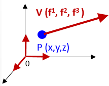
Visualization of a vector field in 3D Euclidean space
The vector field at the point P(x,y,z) is defined as the tuple (f1(x,y,z), f2(x,y,z), f3(x,y,z)). The vector over a field of n dimension field and basis vectors {ei} can be formally defined as \[f: \boldsymbol{x} \,\, \epsilon \,\,\, \mathbb{R}^{n} \mapsto \mathbb{R} \\ f(\mathbf{x})=\sum_{i=1}^{n}{f^{i}}(\mathbf{x}).\mathbf{e}_{i}\] Example for 3 dimension space: \[f(x,y,z) = (2x+z^{3})\boldsymbol{\mathbf{\overrightarrow{i}}} + (xy+e^{-y}-z^{2})\boldsymbol{\mathbf{\overrightarrow{j}}} + \frac{x^{3}}{y}\boldsymbol{\mathbf{\overrightarrow{k}}}\] Let's carry out the creation of this vector field, f, in SymPy and compute its value at f(1.0, 2.0, 0.5). To begin, we need to establish a 3D coordinate system, denoted as r, and then express the vector using r.
from sympy.vector import CoordSys3Dfrom sympy import exp
r = CoordSys3D('r')
f = (2*r.x + r.z**3)*r.i + (r.x*r.y+sympy.exp(-r.y)-r.z**2)*r.j + (r.x**3/r.y)*r.k
w = f.evalf(subs={r.x: 1.0, r.y: 2.0, r.z: 0.2})
print(w)                                 # 2.008*r.i + 2.09533528323661*r.j + 0.5*r.k
Now, let's consider the same vector V with a second reference; origin 0' and basis vector e'i

Visualization of two coordinate systems
\[f(\mathbf{x})=\sum_{i=1}^{n} f'^{i}(\mathbf{x}).\mathbf{e'}_{i}\] The transformation matrix Sij convert the coordinates value functions fi and f'i. The tuple f =(fi) is the co-vector field for the vector field V
\[S_{ij}: \begin{Vmatrix} f^{1} \\ f^{2} \\ f^{3} \end{Vmatrix} \mapsto \begin{Vmatrix} f'^{1} \\ f'^{2} \\ f'^{3} \end{Vmatrix}\] The scalar product of the co-vector f' and vector v(f)
Differential operators
Let's demonstrate how to calculate differential operators using the SymPy library within a 3D Cartesian coordinate system. To begin, we'll create a class named DiffOperators which will encapsulate the implementation of various differential operators and transforms.
Gradient
Consider a scalar field f
class DiffOperators(object):
    def __init__(self, expr: Expr):
        self.expr = expr

    def gradient(self) -> VectorZero:
        from sympy.vector import gradient
return gradient(self.expr, doit=True)Example of input function: \[f(x,y,z)=x^{2}yz\]
r = CoordSys3D('r')
this_expr = r.x*r.x*r.y*r.z
diff_operator = DiffOperators(this_expr)
grad_res = diff_operator.gradient()
\[\triangledown f(x,y,z) = 2xyz.\vec{i} + x^{2}z.\vec{j} + x^{2}y.\vec{k}\]
Divergence
Divergence is a vector operator used to quantify the strength of a vector field's source or sink at a specific point, producing a signed scalar value. When applied to a vector F, comprising components X, Y, and Z, the divergence operator consistently yields a scalar result [ref 6].
\[div(F)=\triangledown .F=\frac{\partial X}{\partial x}+\frac{\partial Y}{\partial y}+\frac{\partial Z}{\partial z}\]
def divergence(self, base_vec: Expr) -> VectorZero:
    from sympy.vector import divergence
    div_vec = self.expr*base_vec
    return divergence(div_vec, doit=True)
Using the same input expression as used for the gradient calculation:
div_res = diff_operator.divergence(r.i + r.j + r.k)
\[div(f(x,y,z)[\vec{i} + \vec{j}+ \vec{k}]) = 2x(y+z+xy)\]
Curl
In mathematics, the curl operator represents the minute rotational movement of a vector in three-dimensional space. This rotation's direction follows the right-hand rule (aligned with the axis of rotation), while its magnitude is defined by the extent of the rotation [ref 6]. Within a 3D Cartesian system, for a three-dimensional vector F, the curl operator is defined as follows:
\[ \triangledown * \mathbf{F}=\left (\frac{\partial F_{z}}{\partial y}- \frac{\partial F_{y}}{\partial z} \right ).\vec{i} + \left (\frac{\partial F_{x}}{\partial z}- \frac{\partial F_{z}}{\partial x} \right ).\vec{j} + \left (\frac{\partial F_{y}}{\partial x}- \frac{\partial F_{x}}{\partial y} \right ).\vec{k} \]
def curl(self, base_vectors: Expr) -> VectorZero:
    from sympy.vector import curl
    curl_vec = self.expr*base_vectors
    return curl(curl_vec, doit=True)
If we use only the two base vectors j and k:
curl_res = diff_operator.curl(r.j+r.k)
\[curl(f(x,y,z)[\vec{j} + \vec{k}]) = x^{2}\left ( z-y \right ).\vec{i}-2xyz.\vec{i}+2xyz.\vec{k}\]
Validation
We can confirm the accuracy of the gradient, divergence, and curl operators implemented in SymPy by utilizing the subsequent formulas: \[curl(\triangledown f))= \triangledown *\left ( \triangledown f\right ) = 0\] and \[\triangledown . curl (F) = \triangledown .\left ( \triangledown * F \right ) = 0\]
grad_res = diff_operator.gradient()
assert(diff_operator.curl(grad_res) ==0)   # Print 0

curl_res = diff_operator.curl(r.i + r.j + r.k)
assert(diff_operator.divergence(curl_res) == 0) # Print 0
Transforms
An integral transform transforms a function from the time domain into its equivalent representation in the frequency domain, as depicted in the following diagram:
The evaluation of SymPy functions follows a two-step process:
- Generate function F in frequency space
- Evaluate output of F for given input values.
Laplace
The Laplace transform is a type of integral transform that changes a function of a real variable (typically time, t) into a function in the s-plane, which is a variable in the complex frequency domain [ref 7].. Specifically, it transforms ordinary differential equations into algebraic ones and converts convolution operations into simpler multiplication. The formulation of the Laplace transform is:\[\mathfrak{L}[f(t)](s)=\int_{0}^{+\inf}f(t).e^{-st}dt\]
def laplace(self):
    from sympy import laplace_transform

    return laplace_transform(self.expr, t, s, noconds=True)
Let's create the Laplace transforms for two basic functions and then calculate the outcomes of these transformed functions in the frequency domain, using the values s=0.5 and a=0.2.
t, s = sympy.symbols('t, s', real=True)
a = sympy.symbols('a', real=True)
diff_operator = DiffOperators(sympy.exp(-a*t))
laplace_func = diff_operator.laplace()
print(Laplace_func.evalf(subs={s:0.5, a:0.2})) # 1.4285\[\int_{0}^{+\inf}e^{-at}.e^{-st}dt = \frac{1}{a+s}\]
diff_operator = DiffOperators(sympy.sqrt(-a*t))
laplace_func = diff_operator.laplace() print(Laplace_func.evalf(subs={s:0.5, a:0.2})) # 1.1209\[\int_{0}^{+\inf}\sqrt{at}.e^{-st}dt = \frac{\sqrt{a\pi}}{2.s^{3/2}}\]
Fourier
Like the Laplace transform, the Fourier transform is another integral transform that translates a function into a version that represents the frequencies contained in the original function. The result of this transformation is a complex-valued function dependent on frequency [ref 8]. Often referred to as the frequency domain representation of the original function, the formulation of the Fourier transform is as follows: \[F(x )=\int_{-\inf}^{+\inf}f(t).e^{-2\pi itx}dt\] The implementation uses the SymPy function fourier_transform which takes the function (self.expr) and x, and k parameters as arguments.
def fourier(self):
   from sympy import fourier_transform
return fourier_transform(self.expr, x, k)
Let's implement the Fourier transforms for two simple functions, exp and sin, and then calculate the outcomes of these transformed functions in the frequency domain with k=0.4
x, k = sympy.symbols('x, k', real=True)
diff_operator = DiffOperators(sympy.exp(-x**2))
fourier_func = diff_operator.fourier()
print(fourier_func.evalf(subs={k: 0.4})) # 0.3654
\[\int_{-\inf}^{+\inf}e^{-t^{2}}.e^{-2\pi itx}dt = \sqrt{\pi}.e^{-2\pi x^{2}}\]
diff_operator = DiffOperators(sympy.sin(x))
diff_operator.fourier()
\[\int_{-\inf}^{+\inf}\sin(t).e^{-2\pi itx}dt = 0\]
Thanks for reading. For comprehensive topics on geometric learning, including detailed analysis, reviews and exercises, subscribe to Hands-on Geometric Deep Learning
References
---------------------------
Patrick Nicolas has over 25 years of experience in software and data engineering, architecture design and end-to-end deployment and support with extensive knowledge in machine learning.
He has been director of data engineering at Aideo Technologies since 2017 and he is the author of "Scala for Machine Learning" Packt Publishing ISBN 978-1-78712-238-3
He has been director of data engineering at Aideo Technologies since 2017 and he is the author of "Scala for Machine Learning" Packt Publishing ISBN 978-1-78712-238-3
No comments:
Post a Comment
Note: Only a member of this blog may post a comment.