
Target audience: Intermediate
Estimated reading time: 7'
Newsletter: Geometric Learning in Python
Tensors and vectors, which depend on coordinate systems, can be perplexing even for seasoned practitioners. The third installment of our Geometric Learning in Python series addresses intrinsic and extrinsic coordinate systems, including a transformation from cartesian to polar coordinates.

What you will learn: How to apply coordinates system and leverage intrinsic and extrinsic geometry.
Notes:
- Environment: Python 3.11, Numpy 1.26.4, Geomstats 2.7.0, Matplotlib 3.8.2
- This article is a follow up to Differentiable Manifolds for Geometric Learning
- Source code available at Github.com/patnicolas/Data_Exploration/manifolds
- To enhance the readability of the algorithm implementations, we have omitted non-essential code elements like error checking, comments, exceptions, validation of class and method arguments, scoping qualifiers, and import statements.
Introduction
In geometry, a coordinate system employs one or more numerical values, known as coordinates, to uniquely identify the location of points or other geometric entities within a manifold, like Euclidean space.
This article is the 3rd installment in our series on Geometric Learning in Python following
- Foundation of Geometric Learning introduces differential geometry as a applied to machine learning and its basic components.
- Differentiable Manifolds for Geometric Learning describes manifold components such as tangent vectors, geodesics with implementation in Python for Hypersphere using the Geomstats library.
This article does not offer a formal explanation of vectors, tensors, or coordinate systems. Readers are strongly recommended to seek out tutorials [ref 1], video series [ref 2], or publications [ref 3, 4] for more detailed information.
Note: Classes ManifoldPoint and HypersphereSpace have been introduced in the previous article [ref 5]
Covariance and contravariance
Contravariant and covariant vectors (or tensors) are fundamental concepts in the field of tensor calculus and differential geometry, used to describe geometric and physical entities in a way that is independent of the coordinate system used.
Note: This section provides a summary of the essential aspects of covariant and contravariant vectors. Readers are highly encouraged to refer to relevant tutorials [ref 6] for a more comprehensive understanding.
Contravariant vectors
Contravariant vectors, also known as tangent vectors, are vectors that transform in the same way as the coordinate system's axes. When the coordinate system is stretched or compressed, the components of a contravariant vector change in the same direction.
If the coordinate system is changed, the components of a contravariant vector transform inversely to the coordinates themselves.
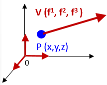
A contravariant vector v is defined by its components vi and its basis vectors e:
\[\vec{v}=\sum_{i=1}^{n} v^{i} \vec{e}_{i}\]Contravariant vectors can be thought of as "pointing" in a certain direction in space, defining directions along which scalar quantities increase.
Covariant vectors
Covariant vectors, or dual vectors, are vectors whose components transform oppositely to the coordinate system's transformation. This means when the coordinate system is stretched, the components of a covariant vector are compressed, and vice versa.
The components of a covariant vector transform in the same way as the coordinate differentials, meaning they scale directly with changes in the coordinate grid.
Covariant vectors are often interpreted as describing surfaces or gradients that interact with other vectors to produce scalar quantities, like the dot product.\[\begin{matrix} \omega : \vec{v} \rightarrow < \ ,\vec{v}>\\ \omega(\vec{v} ) = <\vec{\omega}, \vec{v} > = \omega.v^{T} \end{matrix}\]
Intrinsic vs extrinsic geometries
Intrinsic coordinates
Intrinsic geometry involves studying objects, such as vectors, based on coordinates (or base vectors) intrinsic to the manifold's point. For example, analyzing a two-dimensional vector on a three-dimensional sphere using the sphere's own coordinates.
Intrinsic geometry is crucial in differential geometry because it allows the study of geometric objects as entities in their own right, independent of the surrounding space. This concept is pivotal in understanding complex geometric structures, such as those encountered in general relativity and manifold theory, where the internal geometry defines the fundamental properties of the space.
Here are key points:
- Internal Measurements: Intrinsic geometry involves measurements like distances, angles, and curvatures that are internal to the manifold or surface.
- Coordinate Independence: Intrinsic coordinates describe points on a geometric object using a coordinate system that is defined on the object itself, rather than in the ambient space.
- Curvature: A fundamental concept in intrinsic geometry is curvature, which describes how a geometric object bends or deviates from being flat. The curvature is intrinsic if it is defined purely by the geometry of the object and not by how it is embedded in a higher-dimensional space.

Extrinsic coordinates
Extrinsic geometry studies objects relative to the ambient Euclidean space in which the manifold is situated, such as viewing a vector on a sphere's surface in three-dimensional space.
Extrinsic geometry in differential geometry deals with the properties of a geometric object that depend on its specific positioning and orientation in a higher-dimensional space. It is concerned with how the object is embedded in this surrounding space and how it interacts with the ambient geometry. It contrasts with intrinsic geometry, where the focus is on properties that are independent of the ambient space, considering only the geometry contained within the object itself. Extrinsic analysis is crucial for understanding how geometric objects behave and interact in larger spaces, such as in the study of embeddings, gravitational fields in physics, or complex shapes in computer graphics.
Here’s what extrinsic geometry involves:
- Embedding: Extrinsic geometry examines how a lower-dimensional object, like a surface or curve, is situated within a higher-dimensional space.
- Extrinsic Coordinates: These are coordinates that describe the position of points on the geometric object in the context of the larger space.
- Normal Vectors: An important concept in extrinsic geometry is the normal vector, which is perpendicular to the surface at a given point. These vectors help in defining and analyzing the object's orientation and curvature relative to the surrounding space.
- Curvature: Extrinsic curvature measures how a surface bends within the larger space.
- Projection and Shadow: Extrinsic geometry also looks at how the object projects onto other surfaces or how its shadow appears in the ambient space.

Fig. 2 Visualization of extrinsic in 3-dimension Euclidean space
Implementation
Manifold and coordinates system
We will illustrate the various coordinates on the hypersphere space we introduced in a previous article Geometric Learning in Python: Manifolds
The structure of data points on a manifold is defined by the class ManifoldPoint described in a previous post ManifoldPoint definition.
# --- Code Snippet 1 -------@dataclassclass ManifoldPoint:id: AnyStrlocation: np.arraytgt_vector: Optional[List[float]] = Nonegeodesic: Optional[bool] = Falseintrinsic: Optional[bool] = Falsedef to_intrinsic(self, space: LevelSet) -> np.array:return space.extrinsic_to_intrinsic_coords(self.location) if not self.intrinsicelse self.locationdef to_extrinsic(self, space: LevelSet) -> np.array:return space.intrinsic_to_extrinsic_coords(self.location) if self.intrinsicelse self.locationdef to_intrinsic_polar(self, space: LevelSet) -> np.array:
intrinsic_coordinates = self.to_intrinsic(space)return ManifoldPoint.__cartesian_to_polar(intrinsic_coordinates)
The class ManifoldPoint has 3 methods to define its location given a coordinate system:
- to_intrinsic: Convert the current location from extrinsic cartesian coordinates (3 dimension) to intrinsic cartesian coordinates (2 dimension) if the flag intrinsic is False
- to_extrinsic: Convert the location from intrinsic cartesian coordinates to extrinsic coordinates if the flag intrinsic is True
- to_intrinsic_polar: Convert the current location from extrinsic cartesian coordinates (3 dimension) to intrinsic polar coordinates (2 dimension) if the flag intrinsic is False
This last method relies on the transformation from Cartesian to Polar coordinate on the tangent plane.
The following figure illustrates the transformation from cartesian coordinates (x, y) to polar coordinates (r, theta)

Fig. 3 Visualization of polar coordinates on 2 dimension surface
Here are the mathematical equations for the transformation from cartesian to polar coordinates.\[\begin{matrix} r=\sqrt{x^{2}+y^{2}}\ \ \ \ x.y > 0\\ \theta = arccos(\frac{x}{r})\ \ if\ y >= 0 \ \ \ -arccos(\frac{x}{r}))\ \ \ if\ y <0 \end{matrix}\]
The following private static method __cartesian_to_polar , which executes the two formulas, is straightforward.
# --- Code Snippet 2 -------def __cartesian_to_polar(cartesian_coordinates: np.array) -> np.array:x = cartesian_coordinates[0]y = cartesian_coordinates[1]# Compute rho, theta from x, yrho = math.sqrt(x ** 2 + y ** 2) // First equationtheta = math.acos(x / rho) if y >= 0.0 else -math.acos(x / rho) // Second equation
return np.array([r, theta])
Next, we will explore how to calculate the mean of multiple points on a manifold, both in Euclidean space and along the geodesic of the manifold in extrinsic coordinates.
Euclidean and Fréchet means
Let's explore how to compute means from the perspective of the extrinsic geometry considering a surface that is embedded in a three-dimensional Euclidean space.

Fig. 4 Visualization of Euclidean mean (extrinsic) and Fréchet mean (intrinsic)
First let's compute the mean of multiple point in the default Euclidean space using comprehensive list and Numpy mean functions
# --- Code Snippet 3 -------def euclidean_mean(manifold_points: List[ManifoldPoint]) -> np.array:return np.mean([manifold_pt.location for manifold_pt in manifold_points], axis=0)
Next we compute the intrinsic mean or Fréchet mean using Geomstats class FrechetMean.
def frechet_mean(self, manifold_pt1: ManifoldPoint, manifold_pt2: ManifoldPoint) -> np.array:from geomstats.learning.frechet_mean import FrechetMeanfrechet_mean = FrechetMean(self.space)x = np.stack((manifold_pt1.location, manifold_pt2.location), axis=0)frechet_mean.fit(x)return frechet_mean.estimate_
Similar to the prior article on Manifolds [ref 7] in this series, we utilize the Hypersphere as our evaluation manifold. In the ensuing implementation, we generate two random points on a Hypersphere, calculate the Euclidean and Fréchet means, and then depict the outcomes using the Matplotlib library.
The execution confirms that euclidean mean does not belong to the manifold (as with fig 4) while the Fréchet mean do.
Note: The HypersphereSpace class, introduced in the previous article [ref 7], encapsulates the essential methods for manipulating the Hypersphere function defined in the Geomstats library.
manifold = HypersphereSpace(True)samples = manifold.sample(2)assert(manifold.belongs(samples[0])) # Is True# 1. Generate points on the Hyperpherevector = [0.8, 0.4, 0.7]manifold_points = [ManifoldPoint(id=f'data{index}', location=sample, tgt_vector=vector, geodesic=False)for index, sample in enumerate(samples)]# 2. Compute mean of two points on the Euclidean spaceeuclidean_mean = manifold.euclidean_mean(manifold_points)assert(manifold.belongs(euclidean_mean)) # Is False# 3. Compute the mean on the manifold geodesicsfrechet_mean = manifold.frechet_mean(manifold_points[0], manifold_points[1])print(f'Euclidean mean: {euclidean_mean}\nFrechet mean: {frechet_mean}')assert (manifold.belongs(frechet_mean)) # Is True# 4. Visualize various data points on the Hyperspherefrechet_pt = ManifoldPoint(id='Frechet mean',location=frechet_mean, tgt_vector=None,geodesic=False)manifold_points.append(frechet_pt)manifold.show_manifold(manifold_points, [euclidean_mean])
Output:
Euclidean mean: [ 0.52305713, -0.39238391, -0.10012601]
Fréchet mean: [ 0.79071656, -0.59317508, -0.15136262]
The method show_manifold [ref 8] is called to display the two original points, data0 and data1, on the hypersphere, along with the Fréchet and Euclidean means. It becomes clear that the Euclidean mean does not reside on the hypersphere.

Fig. 5 Illustration of Fréchet and Euclidean mean on a Hypersphere
Intrinsic cartesian coordinates
In the previous article, we explored tangent space and tangent vectors [ref 9] for the hypersphere using extrinsic coordinates. The figure below demonstrates the tangent space, showing both the Euclidean cartesian coordinates X, Y, Z, and the intrinsic cartesian coordinates x, y.

Fig. 6 Visualization of intrinsic cartesian coordinates on a hypersphere
The method extrinsic_to_intrinsic transforms the position of a list of points on the hypersphere from extrinsic cartesian coordinates to intrinsic coordinates. Conversely, the method intrinsic_to_extrinsic changes their location from intrinsic cartesian coordinates to extrinsic coordinates.
def extrinsic_to_intrinsic(self, manifold_pts: List[ManifoldPoint]) -> List[ManifoldPoint]:return [ManifoldPoint(id=pt.id,location=pt.to_intrinsic(self.space),tgt_vector=pt.tgt_vector,geodesic=pt.geodesic,intrinsic=True) for pt in manifold_pts]def intrinsic_to_extrinsic(self, manifold_pts: List[ManifoldPoint]) -> List[ManifoldPoint]:return [ManifoldPoint(id=pt.id,location=pt.to_extrinsic(self.space),tgt_vector=pt.tgt_vector,geodesic=pt.geodesic,intrinsic=False) for pt in manifold_pts]
The code snippet below transforms two randomly chosen points on the hypersphere from extrinsic coordinates (3-dimensional) to intrinsic coordinates (2-dimensional) and then back to extrinsic coordinates.
intrinsic = Falsemanifold = HypersphereSpace(True, intrinsic)# Create Manifold points with default extrinsic coordinatesrandom_samples = manifold.sample(2)manifold_pts = [ManifoldPoint(f'id{index}', value, None, False, intrinsic)for index, value in enumerate(random_samples)]print(f'Extrinsic coordinates:\n{[m_pt.location for m_pt in manifold_pts]}')intrinsic_pts = manifold.extrinsic_to_intrinsic(manifold_pts)print(f'Intrinsic coordinates:\n{[m_pt.location for m_pt in intrinsic_pts]}' )extrinsic_manifold_pts = manifold.intrinsic_to_extrinsic(intrinsic_manifold_pts)
print(f'Regenerated extrinsic coordinates:\n{[m_pt.location for m_pt in extrinsic_manifold_pts]}')
Output:
Extrinsic coordinates:
[[-0.53207445, -0.68768687, 0.49394691],
[-0.45305036, -0.1875893 , -0.87152489]]
Intrinsic Coordinates:
[[1.05417307, 4.05388149],
[2.62909989, 3.53415928)]
Regenerated extrinsic coordinates:
[[-0.53207445, -0.68768687, 0.49394691],
[-0.45305036, -0.1875893 , -0.87152489]]
As expected the final output of the coordinates of the two points matches the original extrinsic coordinates.
Intrinsic polar coordinates
The figure below demonstrates the tangent space, showing both the Euclidean cartesian coordinates X, Y, Z, and the intrinsic cartesian coordinates r, theta.

The extrinsic_to_intrinsic_polar method functions similarly to extrinsic_to_intrinsic for cartesian coordinates. It changes the location of a set of points on the hypersphere from extrinsic cartesian coordinates to intrinsic polar coordinates.
def extrinsic_to_intrinsic_polar(self, manifold_pts: List[ManifoldPoint]) -> List[ManifoldPoint]:return [ManifoldPoint(id=pt.id,location=pt.to_intrinsic_polar(self.space),tgt_vector=pt.tgt_vector,geodesic=pt.geodesic,intrinsic=False) for pt in manifold_pts]
Output:
To extrinsic: [0.25934338 0.14167993 0.95533649]
To intrinsic: [2.09057978 3.26478145]
To polar: [3.16428762 0.64002724]

