

What you will learn: How to approximate PCA on a manifold using Eigen decomposition (orthonormal basis) on the tangent space.
Notes:
- Environments: Python 3.12.5, GeomStats 2.8.0, Matplotlib 3.9, Numpy 2.2.0, Scikit-learn 1.6.0
- Source code is available on GitHub [ref 1]
- To enhance the readability of the algorithm implementations, we have omitted non-essential code elements like error checking, comments, exceptions, validation of class and method arguments, scoping qualifiers, and import statement.
Introduction
This post is a follow-up to the Fréchet Centroid on Manifolds article [ref 2]
Principal Components Analysis (PCA)
Principal Component Analysis (PCA) is a dimensionality reduction technique in machine learning that simplifies large datasets into smaller sets while preserving key patterns and trends.
The PCA process can be summarized in five steps [ref 3]:
- Standardize the Data: Normalize the range of the original continuous variables.
- Calculate the Covariance Matrix: Identify correlations between variables.
- Determine Eigenvectors and Eigenvalues: Compute these from the covariance matrix to identify the principal components.
- Form the Feature Vector: Select the principal components to retain.
- Reproject the Data: Transform the data along the axes of the principal components.

Fig. 1 Visualization of principal components in 3D Euclidean space
Note: These five steps are implemented (and abstracted) in the Scikit-learn Python library within the decomposition.PCA class.
PCA has some serious limitations:
- Assumption of linear relationship: PCA only captures linear correlations between features.
- Sensitivity to scaling: Features with larger ranges dominate the principal components.
- Sensitivity to noise: Noise and outliers can distort the features set
- Sensitivity to missing data: It requires some level of amputation
- Assumption of Gaussian distribution
- Unsupervised learning: It ignores class labels making unsuitable to classification
- Assumption of feature importance: All features have the same importance or weights.
PCA for manifolds
The representation of points on the manifold as tangent vectors at a reference point to fit any machine learning algorithm. The principal components analysis is no exception.
The tangent space is a linear approximation of the manifold at a specific point (usually the Fréchet centroid of the data on the manifold [ref 2] ).
By projecting data onto the tangent space, PCA can be applied as if the data were in Euclidean space.
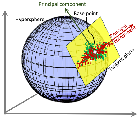
Fig. 2 Visualization of principal components in locally Euclidean tangent plane
PCA on the tangent space provides a way to represent manifold-valued data in a lower-dimensional, Euclidean space for tasks such as visualization, clustering, or regression. It enables the application of statistical analysis tools and tests requiring a Euclidean space.
This approach has numerous benefits
- It allows handling of non-Euclidean data
- It linearizes the manifold locally, reducing the computation complexity entailed by a manifold
- The covariance is intrinsic to the manifold.
Implementation
Components
The goal is to develop a representation and programming framework capable of handling both linear PCA (Euclidean) and locally linear PCA (Manifold).
Let's begin by defining a class, PrincipalComponents, to represent components for both Euclidean spaces and manifolds.
The class attributes include:
The class attributes include:
- base_point: A point on the manifold corresponding to the tangent space, locally Euclidean, where the principal components are calculated.
- Components: A NumPy array representing the principal components.
@dataclass
class PrincipalComponents:
    base_point: np.array
    components: np.array
Next, we define a class, ManifoldPCA, which supports Principal Component Analysis (PCA) for manifolds embedded in a 3D ambient Euclidean space.
The class includes two attributes:
- space: Represents the space type, which can either inherit from `Manifold` (with a locally Euclidean tangent space at a base point) or be `Euclidean` (globally Euclidean, where the base point can be any point in 3D space).
- tgt_pca: Specifies the PCA computation class, which can be either Geomstats tangentPCA or Scikit-learn's PCA class.
The three main methods are:
- estimate: Computes the principal components for a set of points on the manifold.
- project: Projects points on the manifold along the principal components (eigenvector transformation).
- geodesics: Visualizes the curves on the hypersphere associated with the principal components.
class ManifoldPCA(object):
    def __init__(self, space: Manifold) -> None:
        from geomstats.learning.pca import TangentPCA
from geomstats.geometry.euclidean import Euclidean from sklearn.decomposition import PCA
self.tgt_pca = TangentPCA(space, n_components=2) \ if not is instance(space, Euclidean) \ else PCA(n_components=3)
self.space = space
def estimate(self, manifold_pts: np.array, base_point: Optional[np.array] = None) -> PrincipalComponents:
def project(self, manifold_pts: np.array) -> np.array:
def geodesics(self, principal_components: PrincipalComponents) -> List[np.array]:
Computation
The estimate method delegates the computation of principal components to either the tangent space (__tangent_pca) or the 3D Euclidean space (__euclidean_pca), depending on the context. It uses the Geomstats TangentPCA.fit [ref 4] method for manifolds or the Scikit-learn PCA.fit [ref 5] method for Euclidean spaces.
In this article we use the Hypersphere [ref 6] as our test manifold.
For PCA in the tangent space, the Fréchet centroid is used as the base point if none is provided. In the 3D Euclidean space, the arithmetic mean serves as the base point.
As expected, PCA in the Euclidean space produces three-dimensional principal components, whereas PCA in the locally Euclidean tangent space results in two-dimensional principal components.
def estimate(self,
                     manifold_pts: np.array,
                     base_point: Optional[np.array] = None) -> PrincipalComponents:
    from geomstats.geometry.euclidean import Euclidean

    return self .__tangent_pca(manifold_pts, base_point) \
if not isinstance(self.space, Euclidean) \ \
else self.__euclidean_pca(manifold_pts, base_point)
""" Compute the principal components on the tangent of the manifold """
def __tangent_pca(self,
                          manifold_pts: np.array,
                          base_point: Optional[np.array] = None) -> PrincipalComponents:
        from geomstats.learning.frechet_mean import FrechetMean

        # If no base points have been defined ... then use the centroid
        if base_point is None:
            frechet_mean = FrechetMean(self.space)
            frechet_mean.fit(X=manifold_pts, y=None)
            base_point = frechet_mean.estimate_
        # Compute the 2-dimension principal components in intrinsic coordinates
        self.pca.fit(manifold_pts, base_point=base_point)
        return PrincipalComponents(base_point, self.pca.components_)
""" Compute the principal components on the Euclidean space """
def __euclidean_pca(self,
                            manifold_pts: np.array,
                            base_point: Optional[np.array]=None) -> PrincipalComponents:
        self.pca.fit(manifold_pts)
        mean = np.mean(manifold_pts, axis=0) if base_point is None else base_point
return PrincipalComponents(mean, self.pca.components_)
The principal components are directions and constitute an orthonormal basis in which different individual dimensions of the data are linearly uncorrelated. The method project redefine the values of the data points in relation of the new orthonormal basis.
def project(self, manifold_pts: np.array) -> np.array:
    return self.tgt_pca.transform(manifold_pts)
The geodesics corresponding to each orthonormal basis are generated for visualization purposes.
def geodesics(self, principal_components PrincipalComponents) -> List[np.array]:
     import geomstats.backend as gs

     # For now, we generate geodesics only for spheres
     if not isinstance(self.space, Hypersphere):
raise GeometricException( f'Cannot extract geodesics from this type of manifold {self.space}' )
# Extract the geodesic for each of the principal components
base_point = principal_components.base_point
geodesics = [self.space.metric.geodesic(initial_point=base_point, initial_tangent_vec=component)
for component in principal_components.omponents]
# Generate a trace of 200 data points for visualization purpose
trace = gs.linspace(-1.0, 1.0, 200)
geodesic_traces = [geodesic(trace) for geodesic in geodesics]
return geodesic_traces
Evaluation
The goal of this evaluation is to compute and visualize the principal components for a set of data points on a hypersphere [ref ], both:
- On the tangent plane at the Fréchet mean using Geomstats.
- In the surrounding 3D Euclidean space using Scikit-learn.
The steps are explained in the comments within the following code snippet.
# 1. Generate random points on the hypersphere
sphere = Hypersphere(dim=2)
X = sphere.random_uniform(n_samples=8)

# 2. Perform principal components analysis on tangent plane of the hypersphere
manifold_pca = ManifoldPCA(sphere)
principal_components = manifold_pca.estimate(X)
print(f'\nPrincipal components for Hypersphere:\n' f'{principal_components.components}')
# 3. Project the feature set on the 2D tangent plane
projected_points = manifold_pca.project(X)
print(f'\nProjected points on tangent space:\n{projected_points}')
# 4. Create and visualize the geodesics associated to the principal components
geodesic_components = manifold_pca.geodesics(principal_components)
# 5. Visualization
hypersphere_plot = HyperspherePlot(X, principal_components.base_point)
hypersphere_plot.show(geodesic_components)
# 6. Apply linear PCA to the data points on hypershoer
euclidean_pca = ManifoldPCA(Euclidean(3))
principal_components = euclidean_pca.estimate(X)
print(f'\nPrincipal components in Euclidean space')
print(principal_components.components)
# 7. Project the features set on the Euclidean space
projected_points = euclidean_pca.project(X)
print(f'\nProjected points in Euclidean space:\n{projected_points}')
PCA for hypersphere data on tangent space
Output:
Principal components for Hypersphere:
[[ 0.37805 -0.21186 -0.90121]
[ 0.74583 0.64640 0.16091]]
[ 0.74583 0.64640 0.16091]]
Projected points on tangent space:
[[ 0.28557 -0.58902]
[-0.98468 0.58031]
[-0.69088 0.13017]
[-1.16979 -0.79723]
[-0.49557 -0.04852]
[-0.08720 0.82096]
[ 1.64977 0.56592]
[ 1.49278 -0.66260]]

Fig. 3 Visualization of random points on a 3D sphere, along with
geodesics PCA and Fréchet mean
The manifold points are projected on the tangent plane then transformed along the two orthonormal basis.

Fig. 4 Visualization of hypersphere data point projected along the 2 orthonormal bases
on the tangent plane
PCA for hypersphere data on Euclidean space
Principal components in Euclidean space:
[[-0.07085 0.00221 0.99742 ]
[ 0.79399 0.60542 0.05505]
[-0.60377 0.79589 -0.04465]]
Projected points in Euclidean space:
[[-0.25303 -0.50401 -0.49961]
[ 0.68800 0.36335 0.29347]
[ 0.64130 0.04860 -0.10587]
[ 0.51994 -0.65668 0.48229]
[ 0.51764 -0.09482 -0.28160]
[ 0.15862 0.71983 -0.18580]
[-1.12479 0.42143 0.22098]
[-1.14769 -0.29770 0.07614 ]]
This final 3D plot illustrates the original 8 data points on the hypersphere, transformed along the three orthonormal bases in Euclidean space.

Fig. 5 Visualization of hypersphere data point projected along the 3 orthonormal bases
in the Euclidean space
Dimension reduction alternatives
There are several alternative algorithms dedicated to non-linear dimension reduction among them:
Kernel Principal Component Analysis (Kernel PCA) extends Principal Component Analysis (PCA) to handle data that is not linearly separable. By applying a kernel function to map the data into a higher-dimensional space, Kernel PCA reveals complex underlying structures in the data [ref 7].
t-SNE is an unsupervised, non-linear technique designed for exploring and visualizing high-dimensional data. It provides insights into how data is structured in higher dimensions by projecting it into two or three dimensions [ref 8].
Uniform Manifold Approximation and Projection (UMAP): leverages research done for Laplacian eigenmaps to tackle the problem of uniform data distributions on manifolds by combining Riemannian geometry with advances in fuzzy simplicial sets [ref 9].
Locally Linear Embedding (LLE) aims to create a lower-dimensional representation of data while preserving the distances within local neighborhoods. It can be viewed as performing a series of local Principal Component Analyses, which are then combined globally to determine the optimal non-linear embedding [ref 10].


