
Target audience: Advanced
Estimated reading time: 7'
Newsletter: Geometric Learning in Python
The Fisher Information Matrix plays a crucial role in various aspects of machine learning and statistics. Its primary significance lies in providing a measure of the amount of information that an observable random variable carries about an unknown parameter upon which the probability depends.

What you will learn: How to estimate and visualize the Fisher information matrix for Normal and Beta distributions on a hypersphere.
Notes:
- Environments: Python 3.10.10, Geomstats 2.7.0
- This article assumes that the reader is somewhat familiar with differential and tensor calculus [ref 1]. Please refer to our previous articles related to geometric learning listed on Appendix.
- Source code is available at Github.com/patnicolas/Data_Exploration/Information Geometry
- To enhance the readability of the algorithm implementations, we have omitted non-essential code elements like error checking, comments, exceptions, validation of class and method arguments, scoping qualifiers, and import statements.
Introduction
This article is the 10th installments of our ongoing series focused on geometric learning. It introduces some basic elements of information geometry as an extension of differential geometry. As with previous articles, we utilize the Geomstats Python library [ref. 2] to implement concepts associated with geometric learning.
Note: Summaries of my earlier articles on this topic can be found in the Appendix
As a reminder, the primary goal of learning Riemannian geometry is to understand and analyze the properties of curved spaces that cannot be described adequately using Euclidean geometry alone.
Here is a synapsis of this article
- Brief introduction to information geometry
- Overview and mathematical formulation of the Fisher information matrix
- Computation of the Fisher metric to Normal and Beta distributions
- Implementation in Python using the Geomstats library
Information geometry
Use cases
Here is a non-exclusive list of application of information geometry
- Statistical Inference: Parameter estimation, hypothesis testing, and model selection (i.e. Bayesian posterior distributions and in the development of efficient sampling algorithms like Hamiltonian Monte Carlo)
- Optimization: Natural gradient descent method uses the Fisher information matrix to adjust the learning rate dynamically, leading to faster convergence compared to traditional gradient descent.
- Finance: Modeling uncertainties and analyzing statistical properties of financial models.
- Machine Learning: Optimization of learning algorithms (i.e. Understanding the EM algorithm used in statistical estimation for latent variable model)
- Neuroscience: Neural coding and information processing in the brain by modeling neural responses as probability distributions.
- Robotics: Development of probabilistic robotics, where uncertainty and sensor noise are modeled using probability distributions.
- Information Theory: Concepts for encoding, compression, and transmission of information.
Fisher information matrix
The Fisher information matrix is a type of Riemannian metric that can be applied to a smooth statistical manifold [ref 4]. It serves to quantify the informational difference between measurements. The points on this manifold represent probability measures defined within a Euclidean probability space, such as the Normal distribution. Mathematically, it is represented by the Hessian of the Kullback-Leibler divergence.
Let's consider a statistical manifold with coordinates (or parameters) θ and its probability density functions over an interval X as follow:\[P= \left \{ p(x, \theta); \ x \in X \ \int_{R}^{} p(x, \theta) dx = 1\right \}\]The Fisher metric is a Riemann metric tensor defined as the expectation of the partial derivative of the negative log likelihood over two coordinates θ.\[g_{ij}(\theta) = -E\left [ \frac{\partial^2\ log\ p(x,\theta) }{\partial \theta_{i}\partial\theta_{j}} \right ] = - \int_{R}^{}{\frac{\partial^2\ log\ p(x,\theta)) }{\partial \theta_{i}\partial\theta_{j}}}p(x, \theta)dx\]
The Fisher information or Fisher-Rao metric quantifies the amount of information in the data regarding a parameter θ. The Fisher-Rao metric, an intrinsic measure, enables the analysis of a finite, n-dimensional statistical manifold M.\[ds=\sum_{i=1}^{p}{\sum_{j=1}^{p}}g_{ij}\theta^{i}\theta^{j}\]
The Fisher metric for the normal distribution θ = {μ, σ} is computed as:\[\mathfrak{I}(\mu, \sigma)=-\textit{E}_{x-p}\begin{bmatrix} \frac{\partial ^2\ log\ p(\theta)}{\partial \mu^2} & \frac{\partial ^2\ log\ p(\theta)}{\partial \mu \partial \sigma} \\ \frac{\partial ^2\ log\ p(\theta)}{\partial \sigma \partial \mu} & \frac{\partial ^2\ log\ p(\theta)}{\partial \sigma^2} \end{bmatrix} = \begin{bmatrix} \sigma^{-2} & 0\\ 0 & 2\sigma^{-2} \end{bmatrix}\]
The Fisher metric for the beta distribution θ = {α, β} is computed as:\[\varphi (z)=\frac{d^2}{dz^2}\ log \ \Gamma (z)\]
\[\mathfrak{I(\alpha,\beta)}=-\textit{E}_{x-p}\begin{bmatrix} \frac{\partial ^2\ log\ p(\theta)}{\partial \alpha^2} & \frac{\partial ^2\ log\ p(\theta)}{\partial \alpha \partial \beta} \\ \frac{\partial ^2\ log\ p(\theta)}{\partial \beta \partial \alpha} & \frac{\partial ^2\ log\ p(\theta)}{\partial \beta^2} \end{bmatrix}\]
\[\mathfrak{I(\alpha,\beta)}=\begin{bmatrix} \varphi(\alpha)-\varphi(\alpha+\beta) & -\varphi(\alpha+\beta)\\ -\varphi(\alpha+\beta) & \varphi(\beta)-\varphi(\alpha+\beta) \end{bmatrix}\]
Implementation
We leverage the following classes defined in the previous articles:
- ManifoldPoint in Riemann Metric & Connection for Geometric Learning - Setup
- HypersphereSpace in Differentiable Manifolds for Geometric Learning - Hypersphere
Let's first define a base class for all distributions to be defined on a hypersphere [ref 5].
class GeometricDistribution(object):
    _ZERO_TGT_VEC = [0.0, 0.0, 0.0]

    def __init__(self) -> None:
        self.manifold = HypersphereSpace(True)
def show_points(self, num_pts: int, tgt_vector: List[float] = _ZERO_TGT_VEC) -> NoReturn:
# Random point generated on the hypersphere manifold_pts = self._random_manifold_points(num_pts, tgt_vector)
# Exponential map used to project the tgt vector on the hypersphere exp_map = self.manifold.tangent_vectors(manifold_pts)
        for v, end_pt in exp_map:
            print(f'Tangent vector: {v} End point: {end_pt}')
        self.manifold.show_manifold(manifold_pts)
The purpose of the method show_points is to display the various data point with optional tangent vector on the hypersphere. The argument num_pts specifies the number of random points to be defined in the hypersphere. The tangent vector is displayed if the argument tgt_vector not defined as the origin (_ZERO_TGT_VECTOR).
Normal distribution
The class NormalHypersphere encapsulates the display of the normal distribution on the hypersphere. The constructor initialized the normal distribution implemented in the Geomstats library.
The method show_distribution display num_pdfs probability density function over a set of num_manifold_pts, manifold points on the hypersphere. This specific implementation uses only two points. The Fisher-Rao metric is computed using the metric.geodesic Geomstats method.
The metric is applied to 100 points along the geodesic between the two points A and B. Finally, the density functions, pdfs are computed by converting the metric values to the NormalDistribution.point_to_pdf Geomstats method.
class NormalHypersphere(GeometricDistribution): from geomstats.information_geometry.normal import NormalDistributions
    def __init__(self) -> None:
        super(NormalHypersphere, self).__init__()
        self.normal = NormalDistributions(sample_dim=1)
def show_distribution(self, num_pdfs: int, num_manifold_pts: int) -> NoReturn:
manifold_pts = self._random_manifold_points(num_manifold_pts) A = manifold_pts[0] B = manifold_pts[1]
# Apply the Fisher metric for the two manifold points # on a Hypersphere
geodesic_ab_fisher = self.normal.metric.geodesic(A.location, B.location)
t = gs.linspace(0, 1, 100)
# Generate the various density functions associated to # the Fisher metric between the two points on the hypersphere
        pdfs = self.normal.point_to_pdf(geodesic_ab_fisher(t))
        x = gs.linspace(0.2, 0.7, num_pdfs)
        for i in range(num_pdfs):
            plt.plot(x, pdfs(x)[i, :]/20.0)   # Normalization factor
        plt.title(f'Normal distribution on Hypersphere')
        plt.show()
Let's plot 2 randomly sampled data points associated with a tangent_vector on Hypersphere (1) then visualize 40 normalized normal probability density distributions (2).
normal_dist = NormalHypersphere()
num_points = 2
tangent_vector = [0.4, 0.7, 0.2]
         # 1. Display the 2 data points on the hypersphere
num_manifold_pts = normal_dist.show_points(num_points,
tangent_vector)
        # 2. Visualize the 40 normal probabilities density functions
num_pdfs = 40
succeeded = normal_dist.show_distribution(num_pdfs, num_points)

Fig. 1 Two random data points on a Hypersphere with their tangent vectors
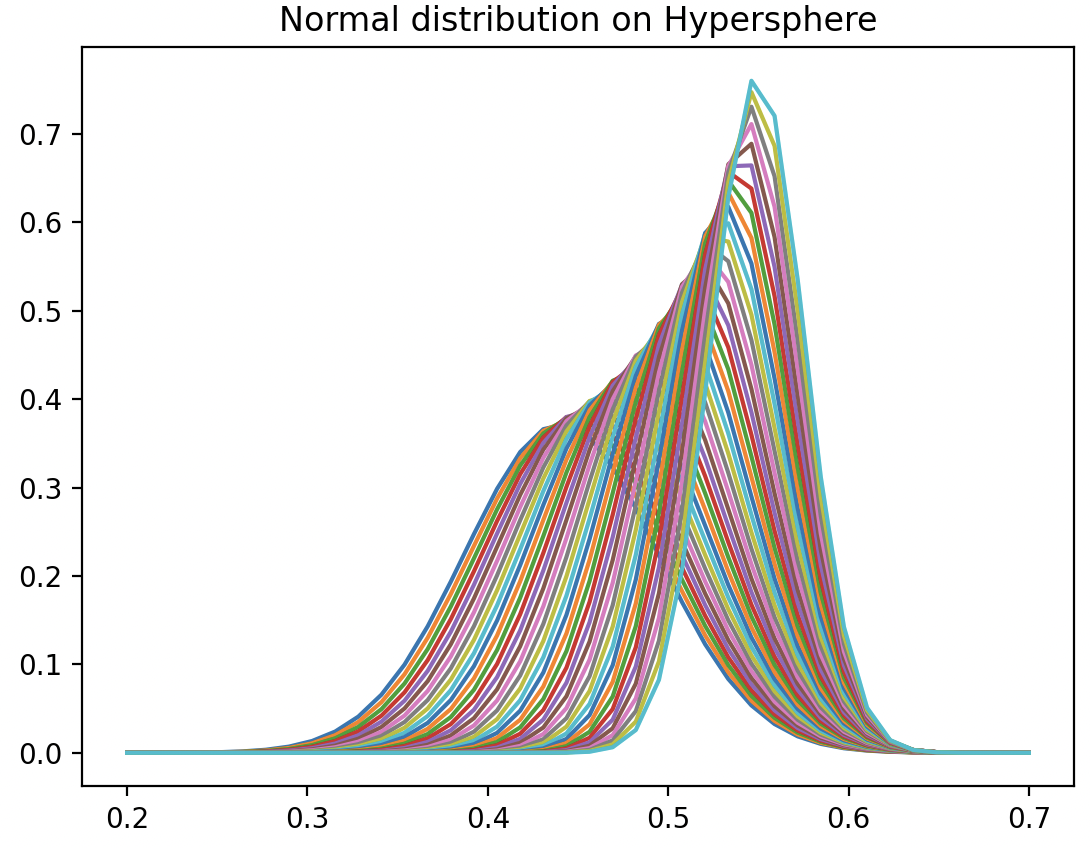
Fig. 2 Visualization of Normal distribution between two random points on a hypersphere
Beta distribution
Let's wrap the evaluation of the Beta distribution on a hypersphere into the class BetaHypersphere that inherits GeometriDistribution. It leverages the BetaDistributions class in Geomstats.
class BetaHypersphere(GeometricDistribution):
   from geomstats.information_geometry.beta import BetaDistributions
def __init__(self) -> None: super(BetaHypersphere, self).__init__()
self.beta = BetaDistributions()
def show_distribution(self, num_manifold_pts: int, num_interpolations: int) -> NoReturn:
        # 1. Generate random points on Hypersphere -Von Mises algorithm
        manifold_pts = self._random_manifold_points(num_manifold_pts)
        t = gs.linspace(0, 1.1, num_interpolations)[1:]
        # 2. Define the beta pdfs associated with each
        beta_values_pdfs = [self.beta.point_to_pdf(manifold_pt.location)(t)
for manifold_pt in manifold_pts]
# 3. Generate, normalize and display each Beta distribution
for beta_values in beta_values_pdfs:
min_beta = min(beta_values)
delta_beta = max(beta_values) - min_beta
y = [(beta_value - min_beta)/delta_beta for beta_value in beta_values] plt.plot(t, y) plt.title(f'Beta distribution on Hypersphere') plt.show()
The method show_distribution generates random points on the Hypersphere (1) and compute the beta density function at these points using the Geomstats BetaDistributions.point_to_pdf (2).
The values generated by the pdfs are normalized then plotted (3)
Let's plot 10 randomly sampled data points on Hypersphere (1) then visualize 200 normalized beta probability density distributions (2).
beta_dist = BetaHypersphere()

num_interpolations = 200
num_manifold_pts = 10
# 1. Display the 10 data points on the hypersphere beta_dist.show_points(num_manifold_pts)
# 2. Visualize the probabilities density functions with# interpolation points
succeeded = beta_dist.show_distribution(num_manifold_pts, num_interpolations)
Fig. 3 10 random data points with on a Hypersphere

Fig. 4 Visualization of Beta distributions associated with 10 data points on hypersphere


