Target audience: Advanced

Estimated reading time: 7'

Posts history

In the realms of healthcare and IT monitoring, I encountered the challenge of managing multiple data points across various variables, features, or observations. Functional data analysis (FDA) is well-suited for addressing this issue.

This article explores how the Hilbert sphere can be used to conduct FDA in non-linear spaces.

Table of contents

Introduction

Functional data analysis

Observation data types

FDA methods

Formal notation

Hilbert sphere

Implementation

Manifold structure

Inner product

Exponential map

Logarithm map

References

What you will learn: Basic concepts of functional data analysis in non-linear spaces through the use of manifolds, along with a hands-on application of Hilbert space using Geomstats in Python.

Notes:

Environments: Python 3.10.10, Geomstats 2.7.0
This article assumes that the reader is somewhat familiar with differential and tensor calculus [ref 1]. Please refer to the previous articles related to geometric learning [ref 2, 3].
Source code is available at Github.com/patnicolas/Data_Exploration/manifolds
To enhance the readability of the algorithm implementations, we have omitted non-essential code elements like error checking, comments, exceptions, validation of class and method arguments, scoping qualifiers, and import statements.'

Introduction

This article provides a summary of functional data analysis and then proceeds to introduce and implement a technique specifically for non-linear manifolds: Hilbert sphere.

This article is the 6th installment in our series on Geometric Learning in Python following

Geometric Learning in Python: Basics introduces differential geometry as an applied to machine learning and its basic components.
Geometric Learning in Python: Manifolds describes manifold components such as tangent vectors, geodesics with implementation in Python for Hypersphere using the Geomstats library.
Geometric Learning in Python: Intrinsic Representation Reviews the various coordinates system using extrinsic and intrinsic representation.
Geometric Learning in Python: Vector and Covector fields describes vector and covector fields with Python implementation in 2 and 3-dimension spaces.
Geometric Learning in Python: Vector Operators illustrates the differential operators, gradient, divergence, curl and laplacian using SymPy library.

Functional data analysis

Functional data analysis (FDA) is a statistical approach designed for analyzing curves, images, or functions that exist within higher-dimensional spaces [ref 4].

Observation data types

Panel Data:

In fields like health sciences, data collected through repeated observations over time on the same individuals is typically known as panel data or longitudinal data. Such data often includes only a limited number of repeated measurements for each unit or subject, with varying time points across different subjects.

Time Series:

This type of data comprises single observations made at regular time intervals, such as those seen in financial markets.

Functional Data:

Functional data involves diverse measurement points across different observations (or subjects). Typically, this data is recorded over consistent time intervals and frequencies, featuring a high number of measurements per observational unit/subjects.

FDA methods

Methods in Functional Data Analysis are classified based on the type of manifold (linear or nonlinear) and the dimensionality or feature count of the space (finite or infinite). The categorization and examples of FDA techniques are demonstrated in the table below.

In Functional Data Analysis (FDA), the primary subjects of study are random functions, which are elements in a function space representing curves, trajectories, or surfaces. The statistical modeling and inference occur within this function space. Due to its infinite dimensionality, the function space requires a metric structure, typically a Hilbert structure, to define its geometry and facilitate analysis.

When the function space is properly established, a data scientist can perform various analytical tasks, including:

Computing statistics such as mean, covariance, and mode
Conducting classification and regression analyses
Performing hypothesis testing with methods like T-tests and ANOVA
Executing clustering
Carrying out inference

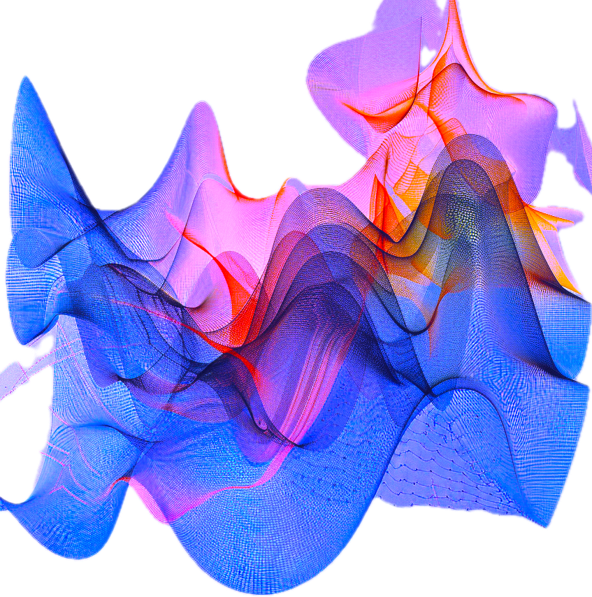
The following diagram illustrates a set of random functions around a smooth function X(tilde) over the interval [0, 1] \[\tilde{X}(t)=3e^{-t^{2}}.sin(25t)-2t^{2}+5 \ \ \ t\in [0, 1]\]

Fig. 1 Visualization of a random functions on Hilbert space

Methods in FDA are classified based on the type of manifold (linear or nonlinear) and the dimensionality or feature count of the space (finite or infinite). The categorization and examples of FDA techniques are demonstrated in the table below.

Manifold

Dimension

Linear

Non-linear

Finite

Euclidean Rn. Rn

Special orthogonal SO(3)

Infinite

Square Integrable

Hilbert sphere

Table 1: Illustration of categorization of FDA techniques

This article focuses on Hilbert space which is specific function space equipped with a Riemann metric (inner product).

Formal notation

Let's consider a sample {x} generated by n Xi random functions as \[x_{i}(t)=X_{i}(t)_{i:1, n} \in \mathbb{R}\ \ \ \ t\in \top \subset \mathbb{R}\]

The function space is a manifold of square integrable functions defined as\[\textit{L}^{2}(T)=\left \{ f: T\rightarrow \mathbb{R}| \int_{T}^{.} f(t)^{T}f(t)dt < \infty \right \}\]The Riemann metric tensor is defined for tangent vectors f and g is induced from and equal to the inner product:\[\left \langle f, g \right \rangle = \int_{T}^{} f(t)^{T}g(t)dt\ \ \ \left \| f \right \| _{\mathit{L}^{2}}=\sqrt{\left \langle f, f \right \rangle} \ \ \ \ (1)\]

Hilbert sphere

Hilbert space is a type of vector space that comes with an inner product, which establishes a distance function, making it a complete metric space. In the context of functional data analysis, attention is primarily given to functions that are square-integrable [ref 5].

Hilbert space has numerous important applications:

Probability theory: The space of random variables centered by the expectation
Quantum mechanics:
Differential equations:
Biological structures: (Protein structures, folds,..)
Medical imaging (MRI, CT-SCAN,...)
Meteorology

The Hilbert sphere S, which is infinite-dimensional, has been extensively used for modeling density functions and shapes, surpassing its finite-dimensional equivalent. This spherical Hilbert geometry facilitates invariant properties and allows for the efficient computation of geometric measures.

The Hilbert sphere is a particular case of function space defined as:\[H(T)=\left \{ f: T\rightarrow \mathbb{R} | \ \ \left \| f \right \|_{L^{2}}= 1 \right \}\]The Riemannian exponential map at p from the tangent space to the Hilbert sphere preserves the distance to origin and defined as:\[exp_{p}(f)=cos\left ( \left \| f \right \|_{E} \right )p+sin\left ( \left \| f \right \|_{E} \right)\frac{f}{\left \| f \right \|_{E}} \ \ \ \ (2) \] where ||f||E is the norm of f in the Euclidean space.

The logarithm (or inverse exponential) map is defined at point p, is defined as \[log_{p}(f)=arccos\left (\left \langle p, f \right \rangle_{p} \right )\frac{f}{\left \| f \right \|} \ \ \ \ (3) \]

Implementation

We will illustrate the various coordinates on the hypersphere space we introduced in a previous article Geometric Learning in Python: Manifolds

We leverage class ManifoldPoint introduced in our previous post, ManifoldPoint definition and used across our series on geometric learning.

As a reminder:

@dataclass
class ManifoldPoint:
    id: AnyStr
    location: np.array
    tgt_vector: List[float] = None
    geodesic: bool = False
    intrinsic: bool = False

Manifold structure

Let's develop a wrapper class named FunctionSpace to facilitate the creation of points on the Hilbert sphere and to carry out the calculation of the inner product, as well as the exponential and logarithm maps related to the tangent space.

Our implementation relies on Geomstats library [ref 6] introduced in Geometric Learning in Python: Manifolds

The function space will be constructed using num_domain_samples, which are evenly spaced real values within the interval [0, 1]. Points on a manifold can be generated using either the Geomstats HilbertSphere.random_point method or by specifying a base point, base_point, and a directional vector.

from geomstats.geometry.functions import HilbertSphere, HilbertSphereMetric


class FunctionSpace(HilbertSphere):
  def __init__(self, num_domain_samples: int):
      domain_samples = gs.linspace(0, 1, num=num_domain_samples)
      super(FunctionSpace, self).__init__(domain_samples, True)

  @staticmethod
  def create_manifold_point(id: AnyStr, vector: np.array, base_point: np.array) -> ManifoldPoint:

    # Compute the tangent vector using the direction 'vector' and point 'base_point'
     tgt_vector =  self.to_tangent(vector, base_point)

     return ManifoldPoint(id, base_point, tgt_vector)

  def random_manifold_points(self, n_samples: int) -> List[ManifoldPoint]: 
     return [ManifoldPoint(
           id=f'rand_{n+1}',
           location=random_pt) 
           for n, random_pt in enumerate(self.random_point(n_samples))]

Let's generate a point on the Hilbert sphere using a random base point on the manifold and a 4 dimension vector.

num_samples = 4
function_space = FunctionSpace(num_samples)
random_base_pt = function_space.random_point()

vector = np.array([1.0, 0.5, 1.0, 0.0])
manifold_pt = function_space.create_manifold_point('id', vector, random_pt)

Output:

Manifold point:

Base point=[[0.13347 0.85738 1.48770 0.29235]],

Tangent Vector=[[ 0.91176 -0.0667 0.01656 -0.19326]],

No Geodesic,

Extrinsic

Inner product

Let's wrap the formula (1) into a method. We introduce the inner_product method to the FunctionSpace class, which serves to encapsulate the call to self.metric.inner_product from the Geomstats method HilbertSphere.inner_product.

This method requires two parameters:

vector_1: The first vector used in the computation of the inner product
vector_2: The second vector used in the computation of the inner product

The second method, manifold_point_inner_product, adds the base point on the manifold without assumption of parallel transport. The base point is origin of both the tangent vector associated with the base point, manifold_base_pt and the tangent vector associated with the second point, manifold_pt.

def inner_product(self, tgt_vector1: np.array, tgt_vector2: np.array) -> np.array:
   return self.metric.inner_product(tgt_vector1,tgt_vector2)

def manifold_point_inner_product(

       self,

       manifold_base_pt: ManifoldPoint,

       manifold_pt: ManifoldPoint) -> np.array:


   return self.metric.inner_product(

               manifold_base_pt.tgt_vector,

               manifold_pt.tgt_vector,
            manifold_base_pt.location)

Let's calculate the inner product of two specific numpy vectors in an 8-dimensional space, using our class, FunctionSpace and focusing on the Euclidean inner product and the norm on the tangent space for one of the vectors.

num_Hilbert_samples = 8
functions_space = FunctionSpace(num_Hilbert_samples)
        
vector1 = np.array([0.5, 1.0, 0.0, 0.4, 0.7, 0.6, 0.2, 0.9])
vector2 = np.array([0.5, 0.5, 0.2, 0.4, 0.6, 0.6, 0.5, 0.5])
inner_prod = functions_space.inner_product(vector1, vector2)
print(f'Inner product of vectors 1 & 2: {str(inner_prod)}')

print(f'Euclidean norm of vector 1: {np.linalg.norm(vector)}')
print(f'Norm of vector 1: {str(math.sqrt(inner_prd))}')

Output:

Inner product of vectors1 & 2: 0.2700

Euclidean norm of vector 1: 1.7635

Norm of vector 1: 0.6071

Exponential map

Let's wrap the formula (2) into a method. We introduce the exp method to the FunctionSpace class, which serves to encapsulate the call to self.metric.exp from the Geomstats method HilbertSphere.exp.

This method requires two parameters:

vector: The directional vector used in the computation the exponential map
manifold_base_pt: The base point on the manifold.

def exp(self, vector: np.array, manifold_base_pt: ManifoldPoint) -> np.array:
   return self.metric.exp(tangent_vec=vector, base_point=manifold_base_pt.location)

Let's compute the exponential map at a random base point on the manifold, for a numpy vector of 8-dimensional, using the class, FunctionSpace.

num_Hilbert_samples = 8
function_space = FunctionSpace(num_Hilbert_samples)

vector = np.array([0.5, 1.0, 0.0, 0.4, 0.7, 0.6, 0.2, 0.9])
assert num_Hilbert_samples == len(vector)
        
exp_map_pt = function_space.exp(vector, function_space.random_manifold_points(1)[0])
print(f'Exponential on Hilbert Sphere:\n{str(exp_map_pt)}')

Output:

Exponential on Hilbert Sphere:

[0.97514 1.6356 0.15326 0.59434 1.06426 0.74871 0.24672 0.95872]

Logarithm map

Let's wrap the formula (3) into a method. We introduce the log method to the FunctionSpace class, which serves to encapsulate the call to self.metric.log from the Geomstats method HilbertSphere.log.

This method requires two parameters:

manifold_base_pt: The base point on the manifold.
target_pt: Another point on the manifold, used to produce the log map.

def log(self, manifold_base_pt: ManifoldPoint, target_pt: ManifoldPoint) ->np.array:
   return self.metric.log(point=manifold_base_pt.location, base_point=target_pt.location)

Let's compute the exponential map at a random base point on the manifold, for a numpy vector of 8-dimensional, using the class, FunctionSpace.

num_Hilbert_samples = 8
function_space = FunctionSpace(num_Hilbert_samples)

random_points = function_space.random_manifold_points(2)
log_map_pt = function_space.log(random_points[0], random_points[1])
print(f'Logarithm from Hilbert Sphere {str(log_map_pt)}')

Output:

Logarithm from Hilbert Sphere

[1.39182 -0.08986 0.32836 -0.24003 0.30639 -0.28862 -0.431680 4.15148]

References

[1] Introduction to Differential Geometry - ETH Zurich

[2] Geometric Learning in Python: Basics

[3] Geometric Learning in Python: Manifolds

[4] Functional Data Analysis - Wikipedia

[5] Principal Component Analysis for Functional Data on Riemannian Manifolds and Spheres

[6] Geomstats - Github

-------------
Patrick Nicolas has over 25 years of experience in software and data engineering, architecture design and end-to-end deployment and support with extensive knowledge in machine learning.
He has been director of data engineering at Aideo Technologies since 2017 and he is the author of "Scala for Machine Learning", Packt Publishing ISBN 978-1-78712-238-3

Sunday, April 7, 2024

Geometric Learning in Python: Functional Data Analysis

Introduction

Functional data analysis

Observation data types

FDA methods

Formal notation

Hilbert sphere

Implementation

Manifold structure

Inner product

Exponential map

Logarithm map

References

No comments:

Post a Comment

Contact Form

Equation Editor

Popular Posts