
Target audience: Intermediate
Estimated reading time: 7'
Estimated reading time: 7'
Intrigued by the idea of applying differential geometry to machine learning but feel daunted?
Our second article in the Geometric Learning in Python series explores fundamental concepts such as manifolds, tangent spaces, and geodesics.

What you will learn: How to implement basic components of manifolds in Python
Notes:
- Environment: Python 3.11, Numpy 1.26.4, Geomstats 2.7.0, Matplotlib 3.8.2
- This article is a follow up to Foundation of Geometric Learning
- Source code available at Github.com/patnicolas/Data_Exploration/manifolds
- To enhance the readability of the algorithm implementations, we have omitted non-essential code elements like error checking, comments, exceptions, validation of class and method arguments, scoping qualifiers, and import statements.
Geometric learning
Geometric learning addresses the difficulties of limited data, high-dimensional spaces, and the need for independent representations in the development of sophisticated machine learning models, including graph-based and physics-informed neural networks.
The following highlights the advantages of utilizing differential geometry to tackle the difficulties encountered by researchers in the creation and validation of generative models [ref 1].
- Understanding data manifolds: Data in high-dimensional spaces often lie on lower-dimensional manifolds. Differential geometry provides tools to understand the shape and structure of these manifolds, enabling generative models to learn more efficient and accurate representations of data.
- Improving latent space interpolation: In generative models, navigating the latent space smoothly is crucial for generating realistic samples. Differential geometry offers methods to interpolate more effectively within these spaces, ensuring smoother transitions and better quality of generated samples.
- Optimization on manifolds: The optimization processes used in training generative models can be enhanced by applying differential geometric concepts. This includes optimizing parameters directly on the manifold structure of the data or model, potentially leading to faster convergence and better local minima.
- Geometric regularization: Incorporating geometric priors or constraints based on differential geometry can help in regularizing the model, guiding the learning process towards more realistic or physically plausible solutions, and avoiding overfitting.
- Advanced sampling techniques: Differential geometry provides sophisticated techniques for sampling from complex distributions (important for both training and generating new data points), improving upon traditional methods by considering the underlying geometric properties of the data space.
- Enhanced model interpretability: By leveraging the geometric structure of the data and model, differential geometry can offer new insights into how generative models work and how their outputs relate to the input data, potentially improving interpretability.
- Physics-Informed Neural Networks: Projecting physics law and boundary conditions such as set of partial differential equations on a surface manifold improves the optimization of deep learning models.
- Innovative architectures: Insights from differential geometry can lead to the development of novel neural network architectures that are inherently more suited to capturing the complexities of data manifolds, leading to more powerful models.
Differential geometry basics
Differential geometry is an extensive and intricate area that exceeds what can be covered in a single article or blog post. There are numerous outstanding publications, including books [ref 2, 3, 4], papers [ref 5] and tutorials [ref 6], that provide foundational knowledge in differential geometry and tensor calculus, catering to both beginners and experts
To refresh your memory, here are some fundamental elements of a manifold:
A manifold is a topological space that, around any given point, closely resembles Euclidean space. Specifically, an n-dimensional manifold is a topological space where each point is part of a neighborhood that is homeomorphic to an open subset of n-dimensional Euclidean space.
Examples of manifolds include one-dimensional circles, two-dimensional planes and spheres, and the four-dimensional space-time used in general relativity.
Differential manifolds are types of manifolds with a local differential structure, allowing for definitions of vector fields or tensors that create a global differential tangent space.
A Riemannian manifold is a differential manifold that comes with a metric tensor, providing a way to measure distances and angles.

Fig 1 Illustration of a Riemannian manifold with a tangent space
A vector field assigns a vector (often represented as an arrow) to each point in a space, lying in the tangent plane at that point. Operations like divergence, which measures the volume change rate in a vector field flow, and curl, which calculates the flow's rotation, can be applied to vector fields.

Given a vector R defined in a Euclidean space Rn and a set of coordinates ci a vector field along the variable lambda is defined: \[\frac{\mathrm{d} \vec{R}}{\mathrm{d} \lambda}=\sum_{i=1}^{n}\frac{\mathrm{d} c^{i}}{\mathrm{d} \lambda}\frac{\partial \vec{R}}{\partial c^i }\] In the case of 2 dimension space, the vector field can be expressed in cartesian (1) and polar (2) coordinates using the Einstein summation convention: \[\frac{\mathrm{d} \vec{R}}{\mathrm{d} \lambda}=\frac{\mathrm{d} x}{\mathrm{d} \lambda}\frac{\partial \vec{R}}{\partial x}+\frac{\mathrm{d} y}{\mathrm{d} \lambda}\frac{\partial \vec{R}}{\partial y} \ \ (1) = \frac{\mathrm{d} r}{\mathrm{d} \lambda}\frac{\partial \vec{R}}{\partial r}+\frac{\mathrm{d} \theta}{\mathrm{d} \lambda}\frac{\partial \vec{R}}{\partial \theta} \ \ (2)\]
Note: While crucial for grasping operations on manifold vector fields, the concepts of covariance and contravariance are outside the purview of this article.
The tangent space at a point on a manifold is the set of tangent vectors at that point, like a line tangent to a circle or a plane tangent to a surface.
Tangent vectors can act as directional derivatives, where you can apply specific formulas to characterize these derivatives.
Given a differentiable function f, a vector v in Euclidean space Rn and a point x on manifold, the directional derivative in v direction at x is defined as: \[\triangledown _{v} f(x)=\sum_{i=1}^{n}v_{i}\frac{\partial f}{\partial x_{i}}(x) \ with \ f: \mathbb{R}^{n} \rightarrow \mathbb{R}\] and the tangent vector at the point x is defined as \[v(f(x\frac{\partial }{\partial x}))=(\triangledown _{v}(f))(x)\]
A geodesic is the shortest path (arc) between two points in a Riemannian manifold.
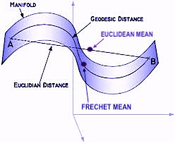
Fig 3 Illustration of manifold geodesics with Frechet mean
Given a Riemannian manifold M with a metric tensor g, the geodesic length L of a continuously differentiable curve f: [a, b] -> M is \[L(f)=\int _a^b \sqrt {g_{f(t))} (\frac{\mathrm{d} f}{\mathrm{d} x}(t), \frac{\mathrm{d} f}{\mathrm{d} x}(t))}dt\]
An exponential map is a map from a subset of a tangent space of a Riemannian manifold. Given a tangent vector v at a point p on a manifold, there is a unique geodesic Gv that satisfy Gv(0)=p and G’v(0)=v. The exponential map is defined as expp(v)= Gv(1)
Intrinsic geometry involves studying objects, such as vectors, based on coordinates (or base vectors) intrinsic to the manifold's point. For example, analyzing a two-dimensional vector on a three-dimensional sphere using the sphere's own coordinates.
Extrinsic geometry studies objects relative to the ambient Euclidean space in which the manifold is situated, such as viewing a vector on a sphere's surface in three-dimensional space.
Geomstats library
Geomstats is a free, open-source Python library designed for conducting machine learning on data situated on nonlinear manifolds, an area known as Geometric Learning. This library offers object-oriented, thoroughly unit-tested features for fundamental manifolds, operations, and learning algorithms, compatible with various execution environments, including NumPy, PyTorch, and TensorFlow [ref 7].
The library is structured into two principal components:
- geometry: This part provides an object-oriented framework for crucial concepts in differential geometry, such as exponential and logarithm maps, parallel transport, tangent vectors, geodesics, and Riemannian metrics.
- learning: This section includes statistics and machine learning algorithms tailored for manifold data, building upon the scikit-learn framework.
Use case: Hypersphere
To enhance clarity and simplicity, we've implemented a unique approach that encapsulates the essential elements of a data point on a manifold within a data class.
An hypersphere S of dimension d, embedded in an Euclidean space d+1 is defined as: \[S^{d}=\left \{ x\in \mathbb{R}^{d+1} \ | \ \left \| x \right \| = 1\right \}\]
Components
First we encapsulate the key components of a point on a manifold into a data class ManifoldPoint for convenience with the following attributes:
- id A label a point
- location A n--dimension Numpy array
- tgt_vector An optional tangent vector, defined as a list of float coordinate
- geodesic A flag to specify if geodesic has to be computed.
- intrinsic A flag to specify if the coordinates are intrinsic, if True, or extrinsic if False.

Fig. 4 Illustration of a ManifoldPoint instance
Note: Description of intrinsic and extrinsic coordinates are not required to understand basic Manifold components and will be covered in a future
# --- Code Snippet 1 ---
@dataclass
class ManifoldPoint:
    id: AnyStr
    location: np.array
    tgt_vector: List[float] = None
    geodesic: bool = False
intrinsic: bool = FalseLet's build a HypersphereSpace as a Riemannian manifold defined as a spheric 3D manifold space of type Hypersphere and a metric hypersphere_metric of type HypersphereMetric.
# --- Code Snippet 3 ---import geomstats.visualization as visualization
from geomstats.geometry.hypersphere import Hypersphere, HypersphereMetric
from typing import NoReturn, List
import numpy as np
import geomstats.backend as gs
class HypersphereSpace(object):
def __init__(self, equip: bool = False, intrinsic: bool=False):
dim = 2
super(HypersphereSpace, self).__init__(dim, intrinsic)
# Geomstats hypersphere self.space = Hypersphere(dim=self.dimension, equip=equip, intrinsic= intrinsic) self.hypersphere_metric = HypersphereMetric(self.space)
    def belongs(self, point: List[float]) -> bool:
        return self.space.belongs(point)
    # Simple uniform sampling
    def sample(self, num_samples: int) -> np.array:
        return self.space.random_uniform(num_samples)
    def tangent_vectors(self, manifold_points: List[ManifoldPoint]) -> List[np.array]:

    def geodesics(self,
                  manifold_points: List[ManifoldPoint],
                  tangent_vectors: List[np.array]) -> List[np.array]:

    def show_manifold(self, manifold_points: List[ManifoldPoint]) -> NoReturn:
The first two methods to generate and validate data point on the manifold are
- belongs to test if a point belongs to the hypersphere
- sample to generate points on the hypersphere using a uniform random generator
Tangent vectors
The method tangent_vectors computes the tangent vectors for a set of manifold point defined with their id, location, vector and geodesic flag. The implementation relies on a simple comprehensive list invoking the nested function tangent_vector (#1). The tangent vectors are computed by projection to the tangent plane using the exponential map associated to the metric hypersphere_metric (#2).
# --- Code Snippet 4 ---
def tangent_vectors(self, manifold_points: List[ManifoldPoint]) -> List[np.array]:

   def tangent_vector(point: ManifoldPoint) -> (np.array, np.array):
        import geomstats.backend as gs
        # Create a tangent vector at the given point on the Manifold
        vector = gs.array(point.tgt_vector)
        tangent_v = self.space.to_tangent(vector, base_point=point.location)
# Compute the end point using the exponential map G(1) =exp_P(v) end_point = self.hypersphere_metric.exp( # 2 tangent_vec=tangent_v, base_point=base_pt ) return tangent_v, end_point
return [self.tangent_vector(point) for point in manifold_points] # 1
This test consists of generating 3 data points, samples on the hypersphere and construct the manifold points through a comprehensive list with a given vector [0.5, 0.3, 0.5] in the Euclidean space and geodesic disabled.
# --- Code Snippet 5 ---
manifold = HypersphereSpace(equip=True)

# Uniform randomly select points on the hypersphere
samples = manifold.sample(3)
# Generate the manifold data points
manifold_points = [
  ManifoldPoint(
    id=f'data{index}',
    location=sample,
    tgt_vector=[0.5, 0.3, 0.5],
    geodesic=False) for index, sample in enumerate(samples)]

# Display the tangent vectors
manifold.show_manifold(manifold_points)
The code for the method show_manifold is described in the Appendix. The execution of the code snippet produces the following plot using Matplotlib.

Fig. 5 Visualization of three random data points and
their tangent vectors on Hypersphere
Geodesics
The geodesics method calculates the trajectory on the hypersphere for each data point in manifold_points, using the tangent_vectors. Similar to how tangent vectors are computed, the determination of geodesics for a group of manifold points is guided by a Python comprehensive list to invoke the nested function geodesic.
# --- Code Snippet 6 ----def geodesics(self,
manifold_points: List[ManifoldPoint],
tangent_vectors: List[np.array]) -> List[np.array]:
def geodesic(manifold_point: ManifoldPoint, tangent_vec: np.array) -> np.array:
return self.hypersphere_metric.geodesic(
initial_point=manifold_point.location,
initial_tangent_vec=tangent_vec
)
return [geodesic(point, tgt_vec)
for point, tgt_vec in zip(manifold_points, tangent_vectors) if point.geodesic]
The geodesic is visualized by plotting 40 intermediate infinitesimal exponential maps created by invoking linspace function as described in Appendix.

Fig. 6 Visualization of two random data points with tangent vectors
and geodesics on Hypersphere

