Showing posts with label manifolds. Show all posts

Monday, January 22, 2024

Differentiable Manifolds for Geometric Learning

Target audience: Intermediate
Estimated reading time: 7'


Intrigued by the idea of applying differential geometry to machine learning but feel daunted? 
Our second article in the Geometric Learning in Python series explores fundamental concepts such as manifolds, tangent spaces, and geodesics.
 
Table of contents
       Components
       Tangent vectors
       Geodesics
Follow me on LinkedIn

What you will learn: How to implement basic components of manifolds in Python

Notes:
  • Environment: Python 3.11, Numpy 1.26.4, Geomstats 2.7.0, Matplotlib 3.8.2
  • This article is a follow up to Foundation of Geometric Learning
  • Source code available at Github.com/patnicolas/Data_Exploration/manifolds
  • To enhance the readability of the algorithm implementations, we have omitted non-essential code elements like error checking, comments, exceptions, validation of class and method arguments, scoping qualifiers, and import statements.

Geometric learning

Geometric learning addresses the difficulties of limited data, high-dimensional spaces, and the need for independent representations in the development of sophisticated machine learning models, including graph-based and physics-informed neural networks.

The following highlights the advantages of utilizing differential geometry to tackle the difficulties encountered by researchers in the creation and validation of generative models [ref 1].
  • Understanding data manifolds: Data in high-dimensional spaces often lie on lower-dimensional manifolds. Differential geometry provides tools to understand the shape and structure of these manifolds, enabling generative models to learn more efficient and accurate representations of data.
  • Improving latent space interpolation: In generative models, navigating the latent space smoothly is crucial for generating realistic samples. Differential geometry offers methods to interpolate more effectively within these spaces, ensuring smoother transitions and better quality of generated samples.
  • Optimization on manifolds: The optimization processes used in training generative models can be enhanced by applying differential geometric concepts. This includes optimizing parameters directly on the manifold structure of the data or model, potentially leading to faster convergence and better local minima.
  • Geometric regularization: Incorporating geometric priors or constraints based on differential geometry can help in regularizing the model, guiding the learning process towards more realistic or physically plausible solutions, and avoiding overfitting.
  • Advanced sampling techniques: Differential geometry provides sophisticated techniques for sampling from complex distributions (important for both training and generating new data points), improving upon traditional methods by considering the underlying geometric properties of the data space.
  • Enhanced model interpretability: By leveraging the geometric structure of the data and model, differential geometry can offer new insights into how generative models work and how their outputs relate to the input data, potentially improving interpretability.
  • Physics-Informed Neural Networks:  Projecting physics law and boundary conditions such as set of partial differential equations on a surface manifold improves the optimization of deep learning models.
  • Innovative architectures: Insights from differential geometry can lead to the development of novel neural network architectures that are inherently more suited to capturing the complexities of data manifolds, leading to more powerful models.
Important NoteIn future articles, we will employ the Geomstats Python library and a use case involving the hypersphere to demonstrate some fundamental concepts of differential geometry.

Differential geometry basics

Differential geometry is an extensive and intricate area that exceeds what can be covered in a single article or blog post. There are numerous outstanding publications, including books [ref 234],  papers [ref 5] and tutorials [ref 6], that provide foundational knowledge in differential geometry and tensor calculus, catering to both beginners and experts 

To refresh your memory, here are some fundamental elements of a manifold:

A manifold is a topological space that, around any given point, closely resembles Euclidean space. Specifically, an n-dimensional manifold is a topological space where each point is part of a neighborhood that is homeomorphic to an open subset of n-dimensional Euclidean space.
Examples of manifolds include one-dimensional circles, two-dimensional planes and spheres, and the four-dimensional space-time used in general relativity.

Differential manifolds are types of manifolds with a local differential structure, allowing for definitions of vector fields or tensors that create a global differential tangent space.

A Riemannian manifold is a differential manifold that comes with a metric tensor, providing a way to measure distances and angles.

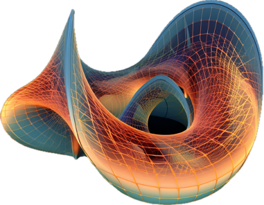
Fig 1 Illustration of a Riemannian manifold with a tangent space


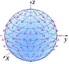
A vector field assigns a vector (often represented as an arrow) to each point in a space, lying in the tangent plane at that point. Operations like divergence, which measures the volume change rate in a vector field flow, and curl, which calculates the flow's rotation, can be applied to vector fields.

Fig 2 Visualization of vector fields on a sphere in 3D space

Given a vector R defined in a Euclidean space Rand a set of coordinates ci a vector field along the variable lambda is defined: \[\frac{\mathrm{d} \vec{R}}{\mathrm{d} \lambda}=\sum_{i=1}^{n}\frac{\mathrm{d} c^{i}}{\mathrm{d} \lambda}\frac{\partial \vec{R}}{\partial c^i }\] In the case of 2 dimension space, the vector field can be expressed in cartesian (1) and polar (2) coordinates using the Einstein summation convention: \[\frac{\mathrm{d} \vec{R}}{\mathrm{d} \lambda}=\frac{\mathrm{d} x}{\mathrm{d} \lambda}\frac{\partial \vec{R}}{\partial x}+\frac{\mathrm{d} y}{\mathrm{d} \lambda}\frac{\partial \vec{R}}{\partial y} \ \ (1) = \frac{\mathrm{d} r}{\mathrm{d} \lambda}\frac{\partial \vec{R}}{\partial r}+\frac{\mathrm{d} \theta}{\mathrm{d} \lambda}\frac{\partial \vec{R}}{\partial \theta} \ \ (2)\]
Note: While crucial for grasping operations on manifold vector fields, the concepts of covariance and contravariance are outside the purview of this article.

The tangent space at a point on a manifold is the set of tangent vectors at that point, like a line tangent to a circle or a plane tangent to a surface.

Tangent vectors can act as directional derivatives, where you can apply specific formulas to characterize these derivatives.

Given a differentiable function f, a vector v in Euclidean space Rand a point x on manifold, the directional derivative in v direction at x is defined as: \[\triangledown _{v} f(x)=\sum_{i=1}^{n}v_{i}\frac{\partial f}{\partial x_{i}}(x) \ with \ f: \mathbb{R}^{n} \rightarrow \mathbb{R}\] and the tangent vector at the point x is defined as \[v(f(x\frac{\partial }{\partial x}))=(\triangledown _{v}(f))(x)\]
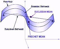
A geodesic is the shortest path (arc) between two points in a Riemannian manifold.

Fig 3 Illustration of manifold geodesics with Frechet mean


Given a Riemannian manifold M with a metric tensor g, the geodesic length L of a continuously differentiable curve  f: [a, b] -> M is \[L(f)=\int _a^b \sqrt {g_{f(t))} (\frac{\mathrm{d} f}{\mathrm{d} x}(t), \frac{\mathrm{d} f}{\mathrm{d} x}(t))}dt\]
An exponential map is a map from a subset of a tangent space of a Riemannian manifold. Given a tangent vector v at a point p on a manifold, there is a unique geodesic Gv that satisfy Gv(0)=p and G’v(0)=vThe exponential map is defined as expp(v)= Gv(1)


Intrinsic geometry involves studying objects, such as vectors, based on coordinates (or base vectors) intrinsic to the manifold's point. For example, analyzing a two-dimensional vector on a three-dimensional sphere using the sphere's own coordinates.

Extrinsic geometry studies objects relative to the ambient Euclidean space in which the manifold is situated, such as viewing a vector on a sphere's surface in three-dimensional space.

Geomstats library

Geomstats is a free, open-source Python library designed for conducting machine learning on data situated on nonlinear manifolds, an area known as Geometric Learning. This library offers object-oriented, thoroughly unit-tested features for fundamental manifolds, operations, and learning algorithms, compatible with various execution environments, including NumPy, PyTorch, and TensorFlow [ref 7].

The library is structured into two principal components:
  • geometry: This part provides an object-oriented framework for crucial concepts in differential geometry, such as exponential and logarithm maps, parallel transport, tangent vectors, geodesics, and Riemannian metrics.
  • learning: This section includes statistics and machine learning algorithms tailored for manifold data, building upon the scikit-learn framework.

Use case: Hypersphere

To enhance clarity and simplicity, we've implemented a unique approach that encapsulates the essential elements of a data point on a manifold within a data class.
An hypersphere S of dimension d, embedded in an Euclidean space d+1 is defined as: \[S^{d}=\left \{ x\in \mathbb{R}^{d+1} \ | \ \left \| x \right \| = 1\right \}\]

Components

First we encapsulate the key components of a point on a manifold into a data class ManifoldPoint for convenience with the following attributes:
  • id A label a point
  • location A n--dimension Numpy array 
  • tgt_vector An optional tangent vector, defined as a list of float coordinate
  • geodesic A flag to specify if geodesic has to be computed.
  • intrinsic A flag to specify if the coordinates are intrinsic, if True, or extrinsic if False.

Fig. 4 Illustration of a ManifoldPoint instance


Note:  Description of intrinsic and extrinsic coordinates are not required to understand basic Manifold components and will be covered in a future 

@dataclass
class ManifoldPoint:
    id: AnyStr
    location: np.array
    tgt_vector: List[float] = None
    geodesic: bool = False
intrinsic: bool = False


Let's build a HypersphereSpace as a Riemannian manifold defined as a spheric 3D manifold space of type Hypersphere and a metric hypersphere_metric of type HypersphereMetric.

import geomstats.visualization as visualization
from geomstats.geometry.hypersphere import Hypersphere, HypersphereMetric
from typing import NoReturn, List
import numpy as np
import geomstats.backend as gs


class HypersphereSpace(GeometricSpace):
    def __init__(self, equip: bool = False, intrinsic: bool=False):
        dim = 2
        super(HypersphereSpace, self).__init__(dim, intrinsic)

coordinates_type = 'intrinsic' if intrinsic else 'extrinsic'
self.space = Hypersphere(dim=self.dimension, equip=equip, 
default_coords_type=coordinates_type)
        self.hypersphere_metric = HypersphereMetric(self.space)


    def belongs(self, point: List[float]) -> bool:
        return self.space.belongs(point)

    def sample(self, num_samples: int) -> np.array:
        return self.space.random_uniform(num_samples)


    def tangent_vectors(self, manifold_points: List[ManifoldPoint]) -> List[np.array]:

    def geodesics(self,
                  manifold_points: List[ManifoldPoint],
                  tangent_vectors: List[np.array]) -> List[np.array]:

    def show_manifold(self, manifold_points: List[ManifoldPoint]) -> NoReturn:


The first two methods to generate and validate data point on the manifold are
  • belongs to test if a point belongs to the hypersphere
  • sample to generate points on the hypersphere using a uniform random generator

Tangent vectors

The method tangent_vectors computes the tangent vectors for a set of manifold point defined with their id, location, vector and geodesic flag. The implementation relies on a simple comprehensive list invoking the nested function tangent_vector (#1). The tangent vectors are computed by projection to the tangent plane using the exponential map associated to the metric hypersphere_metric (#2).

def tangent_vectors(self, manifold_points: List[ManifoldPoint]) -> List[np.array]:
 
   def tangent_vector(point: ManifoldPoint) -> (np.array, np.array):
        import geomstats.backend as gs

        vector = gs.array(point.tgt_vector)
        tangent_v = self.space.to_tangent(vector, base_point=point.location)
        end_point = self.hypersphere_metric.exp(            # 2
               tangent_vec=tangent_v, 
               base_point=point.location)
        return tangent_v, end_point

   return [self.tangent_vector(point) for point in manifold_points]     # 1


This test consists of generating 3 data points, samples on the hypersphere and construct the manifold points through a comprehensive list with a given vector [0.5, 0.3, 0.5] in the Euclidean space and geodesic disabled.

manifold = HypersphereSpace(True)

# Uniform randomly select points on the hypersphere
samples = manifold.sample(3)
# Generate the manifold data points   
manifold_points = [
  ManifoldPoint(
    id=f'data{index}',
    location=sample,
    tgt_vector=[0.5, 0.3, 0.5],
    geodesic=False) for index, sample in enumerate(samples)]

# Display the tangent vectors
manifold.show_manifold(manifold_points)

The code for the method show_manifold is described in the Appendix. The execution of the code snippet produces the following plot using Matplotlib.
Fig. 5 Visualization of three random data points and 
their tangent vectors on Hypersphere
 

Geodesics

The geodesics method calculates the trajectory on the hypersphere for each data point in manifold_points, using the tangent_vectors. Similar to how tangent vectors are computed, the determination of geodesics for a group of manifold points is guided by a Python comprehensive list to invoke the nested function geodesic.

def geodesics(self,
         manifold_points: List[ManifoldPoint],
         tangent_vectors: List[np.array]) -> List[np.array]:
  
    def geodesic(manifold_point: ManifoldPoint, tangent_vec: np.array) -> np.array:
          return self.hypersphere_metric.geodesic(
               initial_point=manifold_point.location,
               initial_tangent_vec=tangent_vec
           )

    return [geodesic(point, tgt_vec)
           for point, tgt_vec in zip(manifold_points, tangent_vectors) if point.geodesic]


The geodesic is visualized by plotting 40 intermediate infinitesimal exponential maps created by invoking linspace function as described in Appendix
Fig. 6 Visualization of two random data points with tangent vectors 
and geodesics on Hypersphere

References

[2] Differential Geometric Structures W. Poor - Dover Publications, New York  1981
[3] Tensor Analysis on Manifolds R Bishop, S. Goldberg - Dover Publications, New York  1980
[4] Introduction to Smooth Manifolds J. Lee - Springer Science+Business media New York 2013

-------------
Patrick Nicolas has over 25 years of experience in software and data engineering, architecture design and end-to-end deployment and support with extensive knowledge in machine learning. 
He has been director of data engineering at Aideo Technologies since 2017 and he is the author of "Scala for Machine Learning", Packt Publishing ISBN 978-1-78712-238-3 
and Geometric Learning in Python Newsletter on LinkedIn.

Appendix

The implementation of the method show_manifold is shown for reference. It relies on the geomstats visualization library. The various components of data points on manifold (location, tangent vector, geodesics) are displayed according to the values of their attributes. Points on 3-dimension Euclidean space are optionally display for reference.

import geomstats.visualization as visualization


def show_manifold(self, 
      manifold_points: List[ManifoldPoint],
      euclidean_points: List[np.array] = None) -> NoReturn:
  import matplotlib.pyplot as plt

  fig = plt.figure(figsize=(10, 10))
  ax = fig.add_subplot(111, projection="3d")
  # Walk through the list of data point on the manifold
  for manifold_pt in manifold_points:
     ax = visualization.plot(
          manifold_pt.location,
                ax=ax,
                space="S2",
                s=100,
                alpha=0.8,
                label=manifold_pt.id)

            # If the tangent vector has to be extracted and computed
     if manifold_pt.tgt_vector is not None:
        tgt_vec, end_pt = self.__tangent_vector(manifold_pt)

        # Show the end point and tangent vector arrow
        ax = visualization.plot(end_pt, ax=ax, space="S2", s=100, alpha=0.8, label=f'End {manifold_pt.id}')
        arrow = visualization.Arrow3D(manifold_pt.location, vector=tgt_vec)
        arrow.draw(ax, color="red")

        # If the geodesic is to be computed and displayed
        if manifold_pt.geodesic:
           geodesics = self.__geodesic(manifold_pt, tgt_vec)

           # Arbitrary plot 40 data point for the geodesic from the tangent vector
           geodesics_pts = geodesics(gs.linspace(0.0, 1.0, 40))
           ax = visualization.plot(
                geodesics_pts,
                ax=ax,
                space="S2",
                color="blue",
                label=f'Geodesic {manifold_pt.id}')

# Display points in Euclidean space of Hypersphere if any specified
if euclidean_points is not None:
for index, euclidean_pt in enumerate(euclidean_points):
ax.plot(
euclidean_pt[
0],
euclidean_pt[
1],
euclidean_pt[
2],
**{
'label': f'E-{index}', 'color': 'black'},
alpha=0.5)

   ax.legend()
   plt.show()

Friday, December 29, 2023

Foundation of Geometric Learning

Target audience: Beginner
Estimated reading time: 4'
NewsletterGeometric Learning in Python   
     
Facing challenges with high-dimensional, densely packed but limited data, and complex distributions? Differential geometry offers a solution by enabling data scientists to grasp the true shape and distribution of data.

Table of contents
      Deep learning
Follow me on LinkedIn

What you will learn: You'll discover how differential geometry tackles the challenges of scarce data, high dimensionality, and the demand for independent representation in creating advanced machine learning models, such as graph or physics-informed neural networks.

Note
This article does not deal with the mathematical formalism of differential geometry or its implementation in Python.


Challenges 

Deep learning

Data scientists face challenges when building deep learning models that can be addressed by differential geometry. Those challenges are:
  • High dimensionality: Models related to computer vision or images deal with high-dimensional data, such as images or videos, which can make training more difficult due to the curse of dimensionality.
  • Availability of quality data: The quality and quantity of training data significantly affect the model's ability to generate realistic samples. Insufficient or biased data can lead to overfitting or poor generalization.
  • Underfitting or overfitting: Balancing the model's ability to generalize well while avoiding overfitting to the training data is a critical challenge. Models that overfit may generate high-quality outputs that are too similar to the training data, lacking novelty.
  • Embedding physics law or geometric constraints: Incorporating domain constraints such as boundary conditions or differential equations model s very challenging for high-dimensional data.
  • Representation dependence: The performance of many learning algorithms is very sensitive to the choice of representation (i.e. z-normalization impact on predictors).

Generative modeling

Generative modeling includes techniques such as auto-encoders, generative adversarial networks (GANs), Markov chains, transformers, and their various derivatives.

Creating generative models presents several specific challenges beyond plain vanilla deep learning models for data scientists and engineers, primarily due to the complexity of modeling and generating data that accurately reflects real-world distributions. The challenges that can be addressed with differential geometry include:
  • Performance evaluation: Unlike supervised learning models, assessing the performance of generative models is not straightforward. Traditional metrics like accuracy do not apply, leading to the development of alternative metrics such as the Frechet Inception Distance (FID) or Inception Score, which have their limitations.
  • Latent space interpretability: Understanding and interpreting the latent space of generative models, where the model learns a compressed representation of the data, can be challenging but is crucial for controlling and improving the generation process.


What is differential geometry

Differential geometry is a branch of mathematics that uses techniques from calculus, algebra and topology to study the properties of curves, surfaces, and higher-dimensional objects in space. It focuses on concepts such as curvature, angles, and distances, examining how these properties vary as one moves along different paths on a geometric object [ref 1]. 
Differential geometry is crucial in understanding the shapes and structures of objects that can be continuously altered, and it has applications in many fields including
physics (I.e., general relativity and quantum mechanics), engineering, computer science, and data exploration and analysis.

Moreover, it is important to differentiate between differential topology and differential geometry, as both disciplines examine the characteristics of differentiable (or smooth) manifolds but aim for different goals. Differential topology is concerned with the overarching structure or global aspects of a manifold, whereas differential geometry investigates the manifold's local and differential attributes, including aspects like connection and metric [ref 2].

In summary differential geometry provides data scientists with a mathematical framework facilitates the creation of models that are accurate and complex by leveraging geometric and topological insights [ref 3].


Applicability of differential geometry

Why differential geometry?

The following highlights the advantages of utilizing differential geometry to tackle the difficulties encountered by researchers in the creation and validation of generative models.

Understanding data manifolds: Data in high-dimensional spaces often lie on lower-dimensional manifolds. Differential geometry provides tools to understand the shape and structure of these manifolds, enabling generative models to learn more efficient and accurate representations of data.

Improving latent space interpolation: In generative models, navigating the latent space smoothly is crucial for generating realistic samples. Differential geometry offers methods to interpolate more effectively within these spaces, ensuring smoother transitions and better quality of generated samples.

Optimization on manifolds: The optimization processes used in training generative models can be enhanced by applying differential geometric concepts. This includes optimizing parameters directly on the manifold structure of the data or model, potentially leading to faster convergence and better local minima.

Geometric regularization: Incorporating geometric priors or constraints based on differential geometry can help in regularizing the model, guiding the learning process towards more realistic or physically plausible solutions, and avoiding overfitting.

Advanced sampling techniques: Differential geometry provides sophisticated techniques for sampling from complex distributions (important for both training and generating new data points), improving upon traditional methods by considering the underlying geometric properties of the data space.

Enhanced model interpretability: By leveraging the geometric structure of the data and model, differential geometry can offer new insights into how generative models work and how their outputs relate to the input data, potentially improving interpretability.

Physics-Informed Neural Networks:  Projecting physics law and boundary conditions such as set of partial differential equations on a surface manifold improves the optimization of deep learning models.

Innovative architectures: Insights from differential geometry can lead to the development of novel neural network architectures that are inherently more suited to capturing the complexities of data manifolds, leading to more powerful and efficient generative models. 

In summary, differential geometry equips researchers and practitioners with a deep toolkit for addressing the intrinsic challenges of generative AI, from better understanding and exploring complex data landscapes to developing more sophisticated and effective models [ref 3].

Representation independence

The effectiveness of many learning models greatly depends on how the data is represented, such as the impact of z-normalization on predictors. Representation Learning is the technique in machine learning that identifies and utilizes meaningful patterns from raw data, creating more accessible and manageable representations. Deep neural networks, as models of representation learning, typically transform and encode information into a different subspace. 
In contrast, differential geometry focuses on developing constructs that remain consistent regardless of the data representation method. It gives us a way to construct objects which are intrinsic to the manifold itself [ref 4].

Manifold and latent space

A manifold is essentially a space that, around every point, looks like Euclidean space, created from a collection of maps (or charts) called an atlas, which belongs to Euclidean space. Differential manifolds have a tangent space at each point, consisting of vectors. Riemannian manifolds are a type of differential manifold equipped with a metric to measure curvature, gradient, and divergence. 
In deep learning, the manifolds of interest are typically Riemannian due to these properties.

It is important to keep in mind that the goal of any machine learning or deep learning model is to predict p(y) from p(y|x) for observed features y given latent features x.\[p(y)=\int_{\Omega }^{} p(y|x).p(x)dx\].The latent space x can be defined as a differential manifold embedding in the data space (number of features of the input data).
Given a differentiable function f on a domain  a manifold of dimension d is defined by:
\[\mathit{M}=f(\Omega) \ \ \ with \ f: \Omega \subset \mathbb{R}^{d}\rightarrow \mathbb{R}^{d}\]
In a Riemannian manifold, the metric can be used to 
  • Estimate kernel density
  • Approximate the encoder function of an auto-encoder
  • Represent the vector space defined by classes/labels in a classifier
A manifold is usually visualized with a tangent space at give point/coordinates.

Illustration of a manifold and its tangent space


The manifold hypothesis states that real-world high-dimensional data lie on low-dimensional manifolds embedded within the high-dimensional space.

Studying data that reside on manifolds can often be done without the need for Riemannian Geometry, yet opting to perform data analysis on manifolds presents three key advantages [ref 5]:
  • By analyzing data directly on its residing manifold, you can simplify the system by reducing its degrees of freedom. This simplification not only makes calculations easier but also results in findings that are more straightforward to understand and interpret.
  • Understanding the specific manifold to which a dataset belongs enhances your comprehension of how the data evolves over time.
  • Being aware of the manifold on which a dataset exists enhances your ability to predict future data points. This knowledge allows for more effective signal extraction from datasets that are either noisy or contain limited data points.

Graph Neural Networks

Graph Neural Networks (GNNs) are a type of deep learning models designed to perform inference on data represented as graphs. They are particularly effective for tasks where the data is structured in a non-Euclidean manner, capturing the relationships and interactions between nodes in a graph.

Graph Neural Networks operate by conducting message passing across a graph, in which features are transmitted from one node to another through the connecting edges (diffusion process). For instance, the concept of Ricci curvature from differential geometry helps to alleviate congestion in the flow of messages [ref 6].

Physics-Informed Neural Networks

Physics-informed neural networks (PINNs) are versatile models capable of integrating physical principles, governed by partial differential equations, into the learning mechanism. They utilize these physical laws as a form of soft constraint or regularization during training, effectively addressing the challenge of limited data in certain engineering applications [ref 7].

Information geometry

Information geometry is a field that combines ideas from differential geometry and information theory to study the geometric structure of probability distributions and statistical models. It focuses on the way information can be quantified, manipulated, and interpreted geometrically, exploring concepts like distance and curvature within the space of probability distributions
This approach provides a powerful framework for understanding complex statistical models and the relationships between them, making it applicable in areas such as machine learning, signal processing, and more [ref 8].


Python libraries for differential geometry

There are numerous open-source Python libraries available, with a variety of focuses not exclusively tied to machine learning or generative modeling:

References

[8] Information Geometry: Near Randomness and Near Independence - 
      K. Arvin, CT Dodson - Springer-Verlag 2008


-------------
Patrick Nicolas has over 25 years of experience in software and data engineering, architecture design and end-to-end deployment and support with extensive knowledge in machine learning. 
He has been director of data engineering at Aideo Technologies since 2017 and he is the author of "Scala for Machine Learning", Packt Publishing ISBN 978-1-78712-238-3 
and Geometric Learning in Python Newsletter on LinkedIn.