Thursday, October 31, 2024

Impact of Linear Activation on Convolution Networks

 Target audience: Beginner
Estimated reading time: 5'


Have you ever wondered how choosing an activation function can influence the performance of a convolutional neural network? 
This article demonstrates the effect of different linear units on the performance and test loss of the classification of MNIST data.


Follow me on LinkedIn

What you will learn: How various activation functions impact the performance of a convolutional neural network.


Notes

  • Environments: Python 3.11,  Matplotlib 3.9, PyTorch 2.4.1
  • Source code is available at github.com/patnicolas/geometriclearning/dl/model/vision
  • To enhance the readability of the algorithm implementations, we have omitted non-essential code elements like error checking, comments, exceptions, validation of class and method arguments, scoping qualifiers, and import statement.

Introduction 

The choice of activation function(s) for a neural network depends on the type of input data (such as images, text, signals, sound, video, etc.). Many machine learning practitioners often default to using the Rectified Linear Unit (ReLU) for convenience. However, exploring alternative activation functions can be beneficial, as it provides insights into their unique properties and their impact on the training quality for a specific model.

The MNIST database [ref 1], which stands for Modified National Institute of Standards and Technology database, is a large collection of handwritten digit images commonly used for training various image processing systems. It is widely employed for training and testing purposes in the field of machine learning.
The MNIST database contains 60,000 training images and 10,000 testing images.

The classification problem consists of identifying any of the 10 handwritten digits.

Our model

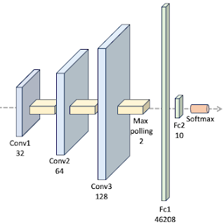
There are various proposed architectures for the training and testing against MNIST data set [ref 2]. We select a 3 layer convolutional neural network followed by two feed forward networks as illustrated below:
Fig. 1 Convolutional Neural Network architecture for MNIST dataset


We utilize the standard network layer configuration for processing the MNIST dataset.

The ConvNet class is implemented as a PyTorch module [ref 3], handling the model's specification, training, and evaluation. Since the activation function is the sole parameter under evaluation in this study, it is provided as a callable function argument in the constructor.
Each digit is represented as a label in this classification model.

class ConvNet(nn.Module):
    num_classes = 10
    
    def __init__(self, activation: Callable[[torch.Tensor], torch.Tensor]) -> None:
        super(ConvNet, self).__init__()

         # Convolutional layers        
        self.conv1 = nn.Conv2d(in_channels=1, out_channels=32, kernel_size=3, stride=1)
        self.bn1 = nn.BatchNorm2d(32)
        
        self.conv2 = nn.Conv2d(in_channels=32, out_channels=64, kernel_size=3, stride=1)
        self.bn2 = nn.BatchNorm2d(64)
        
        self.conv3 = nn.Conv2d(in_channels=64, out_channels=128, kernel_size=3, stride=1)
        self.bn3 = nn.BatchNorm2d(128)

        # Drop out shared by all layers
        self.dropout = nn.Dropout(0.15)

        # Fully connected layers    
        in_fc = 46208
        self.fc1 = nn.Linear(in_features=in_fc, out_features=128)
        self.fc2 = nn.Linear(in_features=128, out_features=ConvNet.num_classes)

         # Activation function shared by all layers
        self.activation = activation
.
For the sake of simplicity, the various layers of the model share the same dropout (regularization) factor and activation function. The forward method implements the flow of data through the 3 convolutional blocks (convolution, batch normalization, max pooling, activation and drop out. 

def forward(self, x: torch.Tensor) -> torch.Tensor:
    # First conv block
    x = self.conv1(x)
    x = self.bn1(x)
    x = F.max_pool2d(x, kernel_size=2)
    x = self.activation(x)
    x = self.dropout(x)
        
    # Second conv block
    x = self.conv2(x)
    x = self.bn2(x)
    x = F.max_pool2d(x, kernel_size=2)
    x = self.activation(x)
    x = self.dropout(x)
        
    # Third conv block
    x = self.conv3(x)
    x = self.bn3(x)
    x = F.max_pool2d(x, kernel_size=2)
    x = self.activation(x)
    x = self.dropout(x)
        
    x = torch.flatten(x, 1)
    # First FFNN block
    x = self.fc1(x)
    x = self.activation (x)
        
    # Last layer with soft max for output [0, 1]
    x = self.fc2(x)
    return F.log_softmax(x, dim=1)


Training and evaluation are performed with the following hyper-parameters:
- Optimizer: Adam
       Learning rate: 0.006
       Momentum: 0.89
- Batch size: 32
- Num of epochs: 10
- train to eval ratio: 0.92
- Normal weight initialization: Disabled
- Loss function: Cross entropy

The reference implementation of the training and evaluation of the convolutional network in PyTorch is shown in the Appendix.

Evaluation

We compare the following four activation functions:
  • Rectified linear unit
  • Leaky rectified linear unit
  • Exponential linear unit
  • Gaussian error linear unit
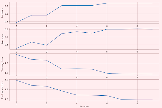
We record and plot the accuracy, precision, training and evaluation loss for the models associated with these activation functions.

Rectified Linear Unit

The Rectified Linear Unit (ReLU), is a widely used activation function in neural networks. It introduces non-linearity into the model, enabling it to learn complex patterns.

Fig. 2 Metrics for Convolutional Network using Rectified Linear Unit - MNIST


Leaky Rectified Linear Unit

Leaky ReLU is a variant of the Rectified Linear Unit (ReLU) activation function used. It address the "dying ReLU" problem, where neurons can stop learning if they consistently output zero. Leaky ReLU introduces a small, non-zero gradient for negative input values, allowing neurons to remain active even when receiving negative inputs.
We use a negative slope of 0.002

Fig. 3 Metrics for Convolutional Network using Leaky Rectifier Linear Unit - MNIST


Exponential Linear Unit

ELU stands for Exponential Linear Unit. It is an activation function used in neural networks as an alternative to ReLU.

Fig. 4 Metrics for Convolutional Network using Exponential Linear Unit - MNIST


Gaussian Error Linear Unit 

The Gaussian Error Linear Unit (GELU) is an activation function popular in transformer architectures (such as BERT and other NLP models)

Fig. 5 Metrics for Convolutional Network using Gaussian Error Linear Unit - MNIST


Analysis

Let's compare the impact of then 4 activation functions on F1 score and evaluation loss.

Fig 6 Impact of selection of activation functions on F1 score for MNIST dataset


The model using exponential linear unit is the only one which F1 score converges quickly to 1.0. All other models have a F1 score of 0.84-0.85. As expected the model ReLU is the slowest to converge.

Fig 7 Impact of selection of activation functions on evaluation loss for MNIST dataset


The loss function profile for the test dataset of each model reflects the previous F1 score plot: the exponential linear unit shows the lowest loss, while the other three models converge toward a similar loss value. ReLU exhibits the slowest convergence profile.

References

[2] Deep Learning Chap 9 Convolutional Networks - I Goodfellow, Y. Bengio, A. Courville - The MIT Press, Cambridge, MA - 2016
[3] Deep Learning with PyTorch Chap 8. Using convolutions to generalize - E. Stevens, L Antiga, T. Viehmann - Manning Publishing, Shelter Island, NY -  2020 


-------------
Patrick Nicolas has over 25 years of experience in software and data engineering, architecture design and end-to-end deployment and support with extensive knowledge in machine learning. 
He has been director of data engineering at Aideo Technologies since 2017 and he is the author of "Scala for Machine Learning", Packt Publishing ISBN 978-1-78712-238-3 and 
Geometric Learning in Python Newsletter on LinkedIn.


Appendix

The typical execution of the training and evaluation of the model is implemented by the '__call__'  dunda method.


def __call__(self,
             train_loader: DataLoader,
             test_loader: DataLoader,
             output_file_name: Optional[AnyStr] = None) -> 
    torch.manual_seed(42)
    initialize_weight(list(model.modules()))

   # Train and evaluation process
   for epoch in range(epochs):
      # Set training mode and execute training
      train_loss = self.__train(epoch, train_loader)

      # Set mode and execute evaluation
      eval_metrics = self.__eval(epoch, test_loader)

Here is a basic implementation of the training function commonly used in PyTorch, for reference.

def __train(self, epoch: int, train_loader: DataLoader) -> float:
   total_loss = 0.0
   # Initialize the gradient for the optimizer
   loss_function = nn.CrossEntropyLoss()
   optimizer = optim.Adam(model.parameters(), learning_rate)

   for features, labels in tqdm(train_loader):
      model.train()
      # Reset the gradient to zero
      for params in model.parameters():
         params.grad = None

         predicted = model(features)  # Call forward - prediction
         raw_loss = loss_function(predicted, labels)
         logging.info(f'Epoch: {epoch} Loss: {raw_loss}')

         raw_loss.backward(retain_graph=True )
         total_loss += raw_loss.data
         optimizer.step()
          
   return total_loss / len(train_loader)

The implementation of the evaluation of the model includes the update and collection of metrics to be plotted.

def __eval(self, epoch: int, test_loader: DataLoader) -> Dict[AnyStr, float]:   
   total_loss = 0
   loss_func = nn.CrossEntropyLoss()
   metric_collector = {}

   # No need for computing gradient for evaluation (NO back-propagation)
   with torch.no_grad():
      for features, labels in tqdm(test_loader):

         model.eval()
         predicted = model(features)
         p = predicted.cpu().numpy()
         l = labels.cpu().numpy()

         for key, metric in metrics.items():
            value = metric(p, l)
            metric_collector[key] = value
            loss = loss_func(predicted, labels)
            total_loss += loss.data

   return metric_collector

Saturday, October 5, 2024

Limitations of the Linear Kalman Filter

 Target audience: Beginner
Estimated reading time: 5'


Frustrated with the results from your Kalman Filter? The issue might be the non-linearity in the process you're modeling. 
This article explores the impact of non-linearity on the accuracy of state predictions made by the linear Kalman filter.


Table of contents
      Theory
      Limitations
      Setup
      Prediction
      Update
      Use case
      Study
Follow me on LinkedIn
What you will learn: The impact of non-linearity of a dynamic process on the accuracy of the state predicted by a linear Kalman filter.

Notes

  • Environments: Python 3.11,  Matplotlib 3.9, Numpy 2.1.2
  • Source code is available at Github.com/patnicolas/Data_Exploration/Filter
  • To enhance the readability of the algorithm implementations, we have omitted non-essential code elements like error checking, comments, exceptions, validation of class and method arguments, scoping qualifiers, and import statement.

Linear Kalman estimator

A deep dive in the underlying assumption and mathematics of Kalman Filter [ref 1] is beyond the scope of this article.

Theory

The linear Kalman filter, sometimes referred as standard Kalman filter is used for systems that can be described by linear state-space models and  assumes that the system’s dynamics and observation models are linear [ref 2].

Fig. 1 Visualization of the Linear Kalman filter algorithm


After initialization, the linear Kalman Filter forecasts the system's state for the upcoming step and estimates the uncertainty associated with this prediction.

Considering An as the state transition model applied to the state xn1, Bn as the control input model applied to the control vector un if it exists, Qn as the covariance of the process noise, and Pn as the error covariance matrix, the forecasted state xis \[\begin{matrix} \widetilde{x}_{n/n-1}=A_{n}.\widetilde{x}_{n-1/n-1} + B_{n}.u_{n} \ \ (1)\\ P_{n/n-1}=A_{n}.P_{n-1/n-1}.A_{n}^{T}+Q_{n} \ \ (2) \end{matrix}\]

Upon receiving a measurement, the Kalman Filter adjusts or corrects the forecast and uncertainty of the current state. It then proceeds to predict future states, continuing this process. 
Thus, with a measurement zn1, a state xn1, and the innovation Sn, the Kalman Gain  and the error covariance are calculated according. \[\begin{matrix} S_{n}=H.P_{n/n-1}.H^{T} +R_{n} \ \ \ \ \  (3)\ \ \ \ \ \ \ \ \ \ \ \ \ \\ G_{n} = \frac{1}{S_{n}}.P_{n/n-1}.H^{T}\ \ \ \ \  (4) \ \ \ \ \ \ \ \ \ \ \ \ \ \ \  \ \ \ \ \ \ \\ \widetilde{x}_{n/n} = \widetilde{x}_{n/n-1}+G_{n}(z_{n}-H.\widetilde{x}_{n/n-1}) \ \ \ (5) \\ g_{n}=I - G_{n}.H \ \ \ \ \ (6) \ \ \ \ \ \ \ \ \ \ \ \ \ \ \ \ \ \ \ \ \ \ \ \ \ \ \ \ \ \ \ \ \ \ \\ P_{n,n}= g_{n}.P_{n/n-1}.g_{n}^{T}+G_{n}.R_{n}.G_{n}^{T} \ \ \ \ (7) \ \ \end{matrix}\]
Fig. 2 Prediction - Update cycle for each measurement

Limitations

The linear Kalman filter is a powerful tool for estimating the state of a linear dynamic system in the presence of uncertainty. However, it has several limitations, particularly when applied to real-world systems that might not perfectly match its assumptions. Here are the key limitations:

  • Assumption of Linearity: The Kalman Filter assumes that both the system dynamics and the measurement processes are linear. The relationship between the current state and the next state and the relationship between the state and the observations should be linear functions.
  • Assumption of Gaussian Noise:  The Kalman Filter assumes that both process noise and measurement noise are Gaussian-distributed with known mean and covariance
  • Strict Accuracy of Models: The Kalman Filter requires an accurate mathematical model of the system (i.e., the transition matrix, control matrix, observation matrix, and their respective noise covariances).
  • Sensitivity to Initial Conditions: The Kalman Filter's performance is sensitive to the choice of initial conditions for the state estimate and error covariance matrix.
  • Time-Invariant Covariance Matrices: The Kalman Filter assumes that the process and measurement noise covariance matrices remain constant over time (or are known in advance if they change)

Implementation

Setup  

The initial step involves programmatically implementing a linear Kalman filter using an object-oriented approach. To achieve this, we define a class named LinearKalmanFilter, which includes two constructors:
  • __init__: This is the default constructor and can be fully specified for a standard linear Kalman filter.
  • build: This alternative constructor is used when there is no control input, and both the process and measurement noise matrices have zero covariance.
The arguments of the constructors defines all the parameter of the Kalman filter:
_x0 : Initial values for the estimated state
_P0 : Initial values for the error covariance matrix
_A : State transition matrix (from state x[n-1] to state x[n])
_H : States to observations (or measurements) matrix
_Q : Process noise covariance matrix
_R : Observation or measurement matrix
_u0 : Optional initial value of the control variables
_B :  Optional control matrix (No control if None)

class LinearKalmanFilter(object):

     # Default constructor for fully defined filter
    def __init__(self,
                 _x0: np.array,
                 _P0: np.array,
                 _A: np.array,
                 _H: np.array,
                 _Q: np.array,
                 _R: np.array,
                 _u0: np.array = None,
                 _B: np.array = None) -> None:
        self.x = _x0
        self.P = _P0
        self.A = _A
        self.H = _H
        self.Q = _Q
        self.R = _R
        self.u = _u0
        self.B = _B


    #   Alternative constructor for the simplified Kalman filter:
    #  - No control input
    #   - No covariance for process and measure noise
    @classmethod
    def build(cls, _x0: np.array, _P0: np.array, _A: np.array, _H: np.array, qr: (float, float)) -> Self:
        dim = len(_x0)
        Q = np.eye(dim)*qr[0]
        R = np.eye(1)*qr[1]
        return cls(_x0, _P0, _A, _H, Q, R)


Prediction

The prediction method, predict, implements the equations (1) and (2) with the process noise w passed as argument.

Note: We are using the Numpy multiplication operator @ instead of numpy.dot method.

def predict(self, w: np.array) -> NoReturn:
     # State:  x[n] = A.x~[n-1] + B.u[n-1] + v
     self.x = self.A @ self.x + w if self.B is None 
                  else self.A @ self.x + self.B @ self.u + w          # Eq (1)
        
    # Error covariance:  P[n] = A[n].P[n-1].A[n]^T + Q[n]
    self.P = self.A @ self.P @ self.A.T + self.Q                    # Eq (2)


Update

The method update from class LinearKalmanFilter implements the computation of innovation and Kalman gain (equations 3 & 4) and update of state, x (equation 5)and error covariance matrix P (equation 7).

def update(self, z: np.array) -> NoReturn:
     # Innovation:  S[n] = H.P[n-1].H^T + R[n]
     S = self.H @ self.P @ self.H.T + R                 # Eq (3)
        
     # Gain: G[n] = P[n-1].H^T/S[n]
     G = self.P @ self.H.T @ np.linalg.inv(S)       # Eq (4)   

     # State estimate y[n] = z[n] - H.x
     y = z - self.H @ self.x
     self.x = self.x + G @ y              # Eq (5)

     # Update error covariance matrix
     g = np.eye(self.P.shape[0]) - G @ self.H        # Eq (6)
     self.P = g @ self.P               # Eq (7)


Evaluation

The objective is to evaluate and quantify the limitation of the Kalman filter for non-linear state update (i.e. x[n] = f(x[n-1]) with f non-linear).

Use case

Our user scenario is the ubiquitous tracking of an object of coordinates x and y on a 2D plan. The plotting {x, y} defines the trajectory in 2D.

\[ x_{k}=x_{k-1}+ \dot{x}_{k-1}.\Delta t+\ddot{x}_{k-1} \frac{(\Delta t^2)}{2} \]
\[ \dot{x}_{k}=\dot{x}_{k-1}+\ddot{x}_{k-1}.\Delta t \]

The derivative  vx = dx/dt (resp. vy = dy/dt) represents the velocity of the object along x (resp. y) axes. The second order derivative d^2x/dt^2 (resp. d^2y/dt^2) defines the acceleration along the x (resp. y) axes.
The force applied to the object is defined as F = m.acceleration, therefore the acceleration is the external control (variable u).
The state prediction can be implemented as the following matrix equation.
\[ x_{k}= \begin{bmatrix} x_{k} \\ y_{k} \\ \dot{x}_{k} \\ \dot{y}_{k} \end{bmatrix} \begin{bmatrix} 1 & 0 & \Delta t & 0  \\ 0 & 1 & 0 & \Delta t \\ 0 & 0 & 1 & 0 \\ 0 & 0 & 0 & 1 \\ \end{bmatrix} x_{k-1}+\begin{bmatrix} \frac{1}{2} (\Delta t)^2 &  0\\ 0 & \frac{1}{2} (\Delta t)^2  \\ \Delta t & 0 \\ 0 & \Delta t \\ \end{bmatrix} \begin{bmatrix} \ddot{x}_{k-1} \\ \ddot{y}_{k-1} \end{bmatrix} \]
The evaluation code initializes the components of the linear Kalman filter, where acceleration serves as the control variable u along with the control matrix B. The simulation, which runs for 200 time steps, with time updates defined as  t[n+1] = t[n] + dt is carried out using the simulate method of class LinearKalmanFilter and described in the appendix.

dt = 0.1
ac = 0.5*dt*dt

# Variables of the linear Kalman Filter
x0 = np.array([[0.0], [np.pi], [0.8], [0.2]])
P0 = np.eye(x0.shape[0])
A = np.array([[1.0, 0.0, dt, 0.0], [0.0, 1.0, 0.0, dt], [0.0, 0.0, 1.0, 0.0], [0.0, 0.0, 0.0, 1.0]])
B = np.array([[ac, 0.0], [0.0, ac], [dt, 0.0], [0.0, dt]])
H = np.array([[1.0, 0.0, 0.0, 0.0], [0.0, 1.0, 0.0, 0.0]])
u = np.array([[1.0], [0.8]])
        
q = 0.6      # Variance for Q process noise matrix
r = 1.0       # Variance for R measurement noise matrix
Q = np.eye(4) * q
R = np.eye(1) * r
      
kf = LinearKalmanFilter(x0, P0, A, H, Q, R, u, B)

num_points = 200
estimation = kf.simulate(num_points,
                                       lambda i: obs_generator_lin(i),
                                       np.array([[0.4], [0.6], [0.1], [0.2]]))


Study

We write 4 functions to generate synthetic observations or measurements for tracking the object {x, y} as follows:
  • f(x) = x
  • f(x) = x*x
  • f(x) = exp(-x/10)
  • f(x) = sqrt(20,000*x)

def obs_generator_lin(i: int) -> np.array:
       return np.array([[i], [i]])
       
def obs_generator_sqr(i: int) -> np.array:
       return np.array([[i], [i*i]])

def obs_generator_exp(i: int) -> np.array:
       return np.array([[i], [math.exp(-i*0.1)]])

def obs_generator_sqrt(i: int) -> np.array:
       return np.array([[i], [math.sqrt(20_000.0*i)]])

The experiment generates 200 values for x-axis [0, 200] for linear and non-linear (sqr(x) = x*x) state update.


Fig. 3 Measured vs estimated trajectory for linear and non-linear (sqr) for state update


Next we plot the trajectory on the 3D plane {x, y} for the 4 generators of observations or measurements.

Fig. 4 Measured vs estimated  2D trajectory over 200 observations for 4 different generators


As expected, in the linear model [x, y = x], the estimated state aligns well with the generated observations (Plot #1). However, in the model [x, y = x^2], the estimated state diverges from the measurements over time (Plot #2), as the compound error grows exponentially. Conversely, for the model [x, y = sqrt{x}], the deviation between the estimated state and measurements decreases over time (Plot #4). In the highly non-linear case (Plot #3), the estimated state fails to keep up with the measurements altogether.


References


-------------
Patrick Nicolas has over 25 years of experience in software and data engineering, architecture design and end-to-end deployment and support with extensive knowledge in machine learning. 
He has been director of data engineering at Aideo Technologies since 2017 and he is the author of "Scala for Machine Learning", Packt Publishing ISBN 978-1-78712-238-3 and 
Geometric Learning in Python Newsletter on LinkedIn.

Appendix

The simulation generates a specified number of measurements (`num_measurements`) using a function or lambda expression, `measure`, which is passed as an argument. At each time step, the process follows these steps:
  1. Generate a measurement,
  2. Predict or estimate the state,
  3. Update the state and error covariance.
def simulate(self,
                 num_measurements: int,
                 measure: Callable[[int], np.array],
                 cov_means: np.array) -> List[np.array]:
   return [self.__estimate_next_state(i, measure, cov_means) for i in range(num_measurements)]


def __estimate_next_state(self, 
          obs_index: int, 
          measure: Callable[[int], np.array], 
          noise: np.array) -> np.array:
    observed = measure(obs_index)      # 1
    self.predict(noise)               # 2
    self.update(observed)        # 3
    return self.x