Showing posts with label Performance. Show all posts

Sunday, September 17, 2023

Compare Python, NumPy and PyTorch Performance

Target audience: Beginner
Estimated reading time: 4'

Recently, I embarked on a healthcare project that involved extracting diagnostic information from Electronic Health Records. While fine-tuning a BERT model, I noticed some atypical latency behaviors. This prompted me to conduct a performance comparison between Python lists, NumPy arrays, and PyTorch tensors.
The implementation relies on a timer decorator to collect latency values.


Table of contents
Follow me on LinkedIn

Notes
  • The implementation uses Python 3.11
  • To enhance the readability of the algorithm implementations, we have omitted non-essential code elements like error checking, comments, exceptions, validation of class and method arguments, scoping qualifiers, and import statements.

Introduction

I assume that most readers are familiar with the various Python, NumPy and PyTorch containers used in this article. But just in case, here is a quick refresh:

Python list
A list in Python is similar to an array in C, C++, Java or Scala except that its elements can have different types.

Python arrays: Array is a container which can hold a fix number of items or elements. Contrary to lists, items of an array should be of the same type. Most of the data structures make use of arrays to implement their algorithms [ref 1].

NumPy arraysA numPy array represents a multidimensional, homogeneous array of fixed-size items. It is implemented as a static buffer of contiguous values of identical types which index can be dynamically modified to generate matrix, tensor or higher dimension numerical structures [ref 2
].

PyTorch tensors: Similarly to numpy array, PyTorch tensors are multi-dimensional arrays containing elements of a single data type. The tensors share the same semantic and operators as NumPy arrays but also support automatic differentiation and support GPU/Cuda math libraries [ref 3].

Timing with decorator

Decorators are very powerful tools in Python since it allows programmers to modify the behavior of a function, method or even a class. Decorators wrap another function in order to extend the behavior of the wrapped function, without permanently modifying it [ref 4].

def timeit(func):
    ''' Decorator for timing execution of methods'''

    def wrapper(*args, **kwargs):
        start = time.time()
        func(*args, **kwargs)
        duration = '{:.3f}'.format(time.time() - start)
        logging.info(f'{args[1]}:{args[3]}\t{duration} secs.')
        return 0

    return wrapper


Benchmark implementation

The objective is to automate the comparison of the various framework and functions by creating a wrapper EvalFunction class.
The evaluation class has two arguments:
  • Descriptive name of the function, func_name used to evaluate the data structures
  • The signature of the function , func used to evaluate the data structures
import array as ar
import time
import numpy as np
from random import Random
from typing import List, AnyStr, Callable, Any, NoReturn
import math
import torch
from dataclasses import dataclass
import logging
from matplotlib import pyplot as plt

collector = {}
@dataclass class EvalFunction: """ Data class for evaluation of Python lists, Array, Numpy array and torch tensor :param func_name Description of the function to execute :param func Lambda to be executed """ func_name: AnyStr func: Callable[[Any], float]  
   def compare(self, input_list: List[float], fraction: float = 0.0) -> NoReturn:
     input_max: int = \
math.floor(len(input_list)*fraction) if 0.0 < fraction <= 1.0 \
else len(input_list)

input_data = input_list[:input_max]

       # Execute lambda through Python list
       self.__execute('python', input_data, 'list:      ')

       # Execute lambda through Python array
       input_array = ar.array('d', input_data)
       self.__execute('python', input_array, 'array:      ')

       # Execute lambda through numpy array
       np_input = np.array(input_list, dtype=np.float32)
       self.__execute('python', np_input, 'lambda: ')

       # Execute native numpy methods
       self.__execute('numpy', np_input, 'native:   ')

       # Execute PyTorch method on CPU
       tensor = torch.tensor(np_input, dtype=torch.float32, device='cpu')
       self.__execute('pytorch', tensor, '(CPU):    ')

       # Execute PyTorch method on GPU
       tensor = torch.tensor(np_input, dtype=torch.float32, device='cuda:0')
       self.__execute('pytorch', tensor, '(CUDA)')


The implementation of the supporting, private method, __execute is described in the Appendix

Evaluation

We've chosen a collection of mathematical transformations that vary in complexity and computational demand to evaluate different frameworks. These transformations involve calculating the mean values produced by the subsequent functions:
\[x_{i}=1+rand{[0, 1]}\]
\[average(x)=\frac{1}{n}\sum_{1}^{n}x_{i}\]
\[sine(x) = average\left ( \sum_{1}^{n}sin\left ( x_{i} \right ) \right )\]
\[sin.exp(x) = average\left ( \sum_{1}^{n}sin\left ( x_{i} \right ) e^{-x_{i}^{2}} \right )\]
\[sin.exp.log(x) = average\left ( \sum_{1}^{n}sin\left ( x_{i} \right ) e^{-x_{i}^{2}} + log(1 + x_{i}))\right )\]

# Functions to evaluate data structures
def average(x) -> float:
    return sum(x)/len(x)
def sine(x) -> float:
    return sum([math.sin(t) for t in x])/len(x)
def sin_exp(x) -> float:
    return sum([math.sin(t)*math.exp(-t) for t in x])/len(x)


# Random value generator
rand = Random(42) num_values = 500_000_000 my_list: List[float] = [1.0 + rand.uniform(0.0, 0.1)] * num_values

# Fraction of the original data set of 500 million data points
fractions = [0.2, 0.4, 0.6, 0.8, 1.0]

# Evaluate the latency for sub data sets of size , len(my_list)*fraction
for fraction in fractions:
eval_average = EvalFunction('sin_exp', average)
eval_average.compare(my_list, fraction)

# x-axis values as size=  len(my_list)*fraction
data_sizes = [math.floor(num_values*fraction) for fraction in fractions]

# Invoke the plotting method
plotter = Plotter(data_sizes, collector)
plotter.plot('Sin*exp 500M')

We conducted the test on an AWS EC2 instance of type p3.2xlarge, equipped with 8 virtual cores, 64GB of memory, and an Nvidia V100 GPU. A basic method for plotting the results is provided in the appendix.

Study 1
We compared the computation time required to determine the {x} -> average{x}  of 500 million real numbers within a Python list, array, NumPy array, and PyTorch tensor.


We compared the computation time required to apply the {x} -> sin{x}.exp{-x} function to 500 million real numbers within a Python list, array, NumPy array, and PyTorch tensor.


Conclusion
  • The performance difference between executing on the GPU versus the CPU becomes more pronounced as the dataset size grows.
  • Predictably, the runtime for both the 'average' and 'sin_exp' functions scales linearly with the size of the dataset when using Python lists or arrays.
  • When executed on the CPU, PyTorch tensors show a 20% performance improvement over NumPy arrays.

Study 2
Le't compare the relative performance of GPU and GPU during the processing of a large PyTorch tensor.
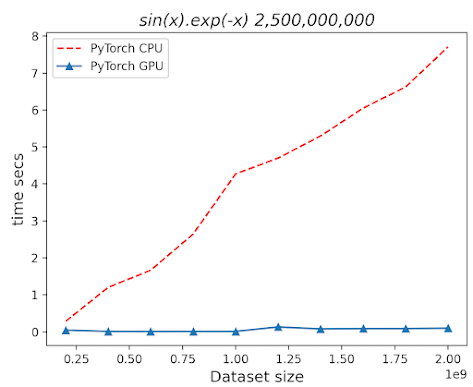

Conclusion
The size of dataset has a very limited impact on the performance of processing PyTorch tensor on GPU while the execution time increases linearly on CPU.

Thank you for reading this article. For more information ...

References


Appendix

The __execute method take two arguments used in the structural pattern match:
  • The framework used to identify the
  • The input data to be processed
The private method __numpy_func applies each the functions (average, sine,...) to a NumPy array, np_array generated from the original list.
The method, __pytorch_func applies each function to a torch tensor derived from np_array.


def __execute(self, framework: AnyStr, input: Any) -> float:
    match framework:
        case 'python':
           return self.func(input)
        case 'numpy':
           return self.__numpy_func(input)
        case 'pytorch':
           return self.__pytorch_func(input)
        case _
           return -1.0


def __numpy_func(self, np_array: np.array) -> float:
   match self.func_name:
      case 'average':
          return np.average(np_array).item()
      case 'sine':
          return np.average(np.sin(np_array)).item()
      case 'sin_exp':
          return np.average(np.sin(np_array)*np.exp(-np_array)).item()


def __pytorch_func(self, tensor: torch.tensor) -> float:
    match self.func_name:
       case 'average':
          return torch.mean(tensor).float()
       case 'sine':
          return torch.mean(torch.sin(tensor)).float()
       case 'sin_exp':
          return torch.mean(torch.sin(tensor) * torch.exp(-tensor)).float()


A simple class, Plotter, to wraps the creation and display of plots using matplotlib.

class Plotter(object):
    markers = ['r--', '^-', '+--', '--', '*-']

    def __init__(self, dataset_sizes: List[int], results_map):
        self.sizes = dataset_sizes
        self.results_map = results_map

    def plot(self, title: AnyStr) -> NoReturn:
        index = 0
        np_sizes = np.array(self.sizes)
        for key, values in self.results_map.items():
            np_values = np.array(values)
            plt.plot(np_sizes, np_values, Plotter.markers[index % len(Plotter.markers)])
            index += 1

        plt.title(title, fontsize=16, fontstyle='italic')
        plt.xlabel('Dataset size', fontsize=13, fontstyle='normal')
        plt.ylabel('time secs', fontsize=13, fontstyle='normal')
        plt.legend(['Python List', 'Python Array', 'Numpy native', 'PyTorch CPU', 'PyTorch GPU'])
        plt.show()


---------------------------
Patrick Nicolas has over 25 years of experience in software and data engineering, architecture design and end-to-end deployment and support with extensive knowledge in machine learning. 
He has been director of data engineering at Aideo Technologies since 2017 and he is the author of "Scala for Machine Learning" Packt Publishing ISBN 978-1-78712-238-3

Sunday, November 1, 2020

Evaluate Performance of Scala Tail Recursion

Target audience: Intermediate
Estimated reading time: 3'

Recursion refers to the technique where a function invokes itself, either directly or indirectly, and such a function is termed a recursive function. 
Some problems can be more effortlessly addressed using recursive algorithms. In this article, we will assess the performance of Scala's tail recursion in comparison to iterative approaches.


Table of contents
Follow me on LinkedIn
   

Overview

In Scala, the tail recursion is a commonly used technique to apply a transformation to the elements of a collection. The purpose of this post is to evaluate the performance degradation of the tail recursion comparatively to iterative based methods.
For the sake of readability of the implementation of algorithms, all non-essential code such as error checking, comments, exception, validation of class and method arguments, scoping qualifiers or import is omitted.

Test benchmark

Let's consider a "recursive" data transformation on an array using a sliding window. For the sake of simplicity, we create a simple polynomial transform on a array of values
   {X0, ... ,Xn, ... Xp}
with a window w, defined as
   f(Xn) = (n-1)Xn-1 + (n-2)Xn-2 + ... + (n-w)Xn-w.  

Such algorithms are widely used in signal processing and technical analysis of financial markets (i.e. moving average, filters).

def polynomial(values: Array[Int]): Int = 
  (if(values.size < W_SIZE) 
     values 
  else 
     values.takeRight(W_SIZE)
  ).sum


The first implementation of the polynomial transform is a tail recursion on each element Xn of the array. The transform f compute f (values(cursor)) from the array values[0, ... , cursor-1] as describe in the code snippet below

 1
 2
 3
 4
 5
 6
 7
 8
 9
10
11
12
13
14
15
16
17
18
19
20
21
22
23
class Evaluation(values: Array[Int]) {
  def recurse(f: Array[Int] => Int): Array[Int] = {

    @scala.annotation.tailrec
    def recurse(
      f: Array[Int] => Int, 
      cursor: Int, 
      results: Array[Int]): Boolean = {  
        
      if( cursor >= values.size) // exit condition
        true
      else {
        val arr = f(values.slice(cursor+1, cursor-W_SIZE))
        results.update(cursor, arr)
        recurse(f, cursor+1, results)
      }
    }

    val results = new Array[Int](values.size)
    recurse(f, 0, results)
    results
  }
}

The second implementation relies on the scanLeft method that return a cumulative of transformed value f(Xn).

def scan(f: Array[Int] => Int): Array[Int] = 
   values.zipWithIndex.scanLeft(0)((sum, vn) => 
         f(values.slice(vn._2+1, vn._2-W_SIZE))
  )

Finally, we implement the polynomial transform on the sliding array window with a map method.

def map(f: Array[Int] => Int): Array[Int] = 
   values.zipWithIndex.map(vn =>  f(values.slice(vn._2+1, vn._2-W_SIZE)))


Performance evaluation

For the test, each of those 3 methods is executed 1000 on a dual core i7 with 8 Gbyte RAM and MacOS X Mountain Lion 10.8. The first test consists of executing the 3 methods and varying the size of the array from 10 to 90. The test is repeated 5 times and the duration is measured in milliseconds.


The tail recursion is significantly faster than the two other methods. The scan methods (scan, scanLeft, scanRight) have significant overhead that cannot be "amortized" over a small array. It is worth noticing that the performance of map and scan are similar. The relative performance of those 3 methods is confirmed while testing with large size array (from 1,000,000 to 9,000,000 items).


Thank you for reading this article. For more information ...

References


---------------------------
Patrick Nicolas has over 25 years of experience in software and data engineering, architecture design and end-to-end deployment and support with extensive knowledge in machine learning. 
He has been director of data engineering at Aideo Technologies since 2017 and he is the author of "Scala for Machine Learning" Packt Publishing ISBN 978-1-78712-238-3

Thursday, June 16, 2016

Analyze Scala Performance Using Javap

Target audience: Beginner
Estimated reading time: 4'

Table of contents
Overview
Follow me on LinkedIn

Overview

As mentioned in a previous post, iterators in Scala, such as foreach, for & while loop have different performance characteristics. A recurrent question between developers is the relative performance of Scala and Java regarding for and while.

The "for comprehension" closure in Scala is indeed a syntactic sugar wraps around a sequence of flatMap and map methods, Monad in Practice. It is expected to be significantly slower and should not be used as an iterator.
We select the higher method foreach to implement the for iterator in Scala.


Note: For the sake of readability of the implementation of algorithms, all non-essential code such as error checking, comments, exception, validation of class and method arguments, scoping qualifiers or import is omitted.

Evaluation

The simple evaluation consists of processing a large number of iterations of a very simple statement which execution does not interfere with the actual performance of the iterator. The code is also is easy to understand. The code for the while loop is described below.

def testRun(numIterations: Int) : Unit = {
  val startTime = System.currentTimeMillis
  var sum: Long = 0
  var i: Int = 0

  while(i < numIterations) {
    var j = 0
    while(j  < 1000) {
      sum += 1
      j += 1
    }
     i += 1
  }
  Console.printf(s"${(System.currentTimeMillis-startTime)}")
}

The test is executed on a 4 cores Intel i7 CPU with java 1.7.02 64-bit and Scala 2.10.2. The chart below, compares the duration of the execution of the for iterator for Java and Scala.


The performance of Scala and Java for executing the while loop are very similar.

The second test consists of comparing the relative performance of Java for loop and Scala foreach higher order method.

def testRun(numIterations: Int) : Unit = {
    var sum: Long = 0
    (0 until numIterations.foreach( sum += _)
}


Analysis using Javap

The first step is to analyze the number of byte-code instructions generated by the Scala compiler. We use the Java Class File Disassembler,  javap, to print out the actual instructions processed by the Java virtual machine.
            javap -c -verbose xxx.class
The sequence of instructions generated for the execution of the while loops are displayed below.

0:   lconst_0
1:   lstore_1
2:   iconst_0
3:   istore_3
4:   iload_3
5:   sipush  1000
8:   if_icmpge       42
11:  iconst_0
12:  istore  4
14:  iload   4
16:  sipush  1000
19:  if_icmpge       35
22:  lload_1
23:  lconst_1
24:  ladd
25:  lstore_1
26:  iload   4
28:  iconst_1
29:  iadd
30:  istore  4
32:  goto    14
35:  iload_3
36:  iconst_1
37:  iadd
38:  istore_3
39:  goto    4
42:  return

Disassembling the Java class for the code with the for iterators produces the following print out:

0:   new     #12; //class scala/runtime/LongRef
3:   dup
4:   lconst_0
5:   invokespecial   #16; //Method scala/runtime/LongRef."<init>":(J)V
8:   astore_1
9:   getstatic       #22; //Field scala/runtime/RichInt$.MODULE$:Lscala/runtime/RichInt$;
12:  getstatic       #27; //Field scala/Predef$.MODULE$:Lscala/Predef$;
15:  iconst_0
16:  invokevirtual   #31; //Method scala/Predef$.intWrapper:(I)I
19:  sipush  1000
22:  invokevirtual   #35; //Method scala/runtime/RichInt$.until$extension0:
                            (II Lscala/collection/immutable/Range;
25:  new             #37; //class JavaScala$$anonfun$testRun$1
28:  dup
29:  aload_0
30:  aload_1
31:  invokespecial   #40; //Method JavaScala$$anonfun$testRun$1."<init>
                          (LJavaScala;Lscala/runtime/LongRef;)V
34:  invokevirtual   #46; //Method scala/collection/immutable/Range.foreach$mVc$sp:
                         (Lscala/Function1;)
37:  return


Although the number of instructions for the for loop is smaller than the number of instructions for while, most of those instructions are function calls:
- conversion of counter to long
- static conversion of int to RichInt to wrap Java Integer:
            @inline implicit def intWrapper(x: Int)= new runtime.RichInt(x)
- ultimately the foreach method is invoked to execute the loop.

Interestingly enough, the foreach method for collection is implemented using the while loop not the for loop. Scala compiler plug-in such as ScalaCL to optimize the execution of iteration on Scala collections, Arrays, Lists,... have been introduced to get around this issue. The reader can also take comfort in using the Java Class File Dissambler to understand how a method or piece of code translate into efficient, or in our case, inefficient byte-code. Quite a few methods in Scala such as foldLeft, reduceLeft uses tail recursion to traverse collections. It would be interesting to compare the relative performance of those methods with alternatives using iterators.. stay tune.

References