Wednesday, March 4, 2015

F-bounded Type Polymorphism

Target audience: Intermediate
Estimated reading time: 4'


This post introduces and describes the concept of bounded polymorphism using self-referential type constraint.


Introduction

F-Bounded Type polymorphism or Bounded Quantification Polymorphism is parametric type polymorphism that constrains the subtypes to themselves using bounds.
Let's consider the following "classification" problem:


How can we guarantee that the SharpPencils bucket contains only sharp pencils, not small pencils or erasers?

Type polymorphism

The first attempt to solve the problem is to rely on parametric type polymorphism. To this purpose, we create a Pencils trait sub-classed by as a bucket for sharp pencils, SharpPencils and a bucket for small pencils, SmallPencils.
For the sake of simplification, we assume that Pencils defines only 2 methods: add (line 4) and pop (line 5) pencils.

1
2
3
4
5
6
7
8
9
trait Pencils[T] {
  private lazy val content = new mutable.ListBuffer[T]
 
  def add(t: T): Unit = content.append(t)
  def pop: List[T] = (content -= data.head).toList
}
 
class SharpPencils extends Pencils[SharpPencils]
class SmallPencils extends Pencils[SmallPencils]


This implementation does not guarantee that SharpPencils is the only bucket that contains the sharp pencils (line 8). Another bucket OtherPencils can be created with sharp pencils, too (line 9).

1
class OtherPencils extends Pencils[SharpPencils]


The solution is to specify constraints (or bounds) on the type of elements contained in each bucket.

Bounded polymorphism

The goal is to make sure that the bucket of specific type (or containing a specific type of pencils). The first step is to make sure that a bucket does not contain other items than a Pencils. This is accomplished by using the recursive (or F-Bound) type polymorphism
   trait A[T]<: ...="" a="" pre="">
The class Pencils is parameterized with one of its sub-type (line 1). None of the existing methods need to change.

1
2
3
4
5
6
trait Pencils[T <: Pencils[T]] {
  private lazy val content = new mutable.ListBuffer[T]
 
  def add(t: T): Unit = content.append(t)
  def pop: List[T] = (content -= data.head).toList
}

This implementation resolve the limitation raised in the previous paragraph. However there is nothing that prevent SharpPencils to contain an eraser or small pencils and SmallPencils to contain sharp pencils, as illustrated in the next code snippet.

// Won't compile!
class SharpPencils extends Pencils[Eraser]
 
 // The following code compiles!
class SharpPencils extends Pencils[SmallPencils]
class SmallPencils extends Pencils[SharpPencils]


Self-referential polymorphism

As a matter of fact, the most effective constraint on a inherited type is the self reference (line 2) that list the type allows for the method to execute.

1
2
3
4
5
6
7
8
9
trait Pencils[T <: Pencils[T]] {
  self: =>
    private lazy val content = new ListBuffer[T]
    def add(t: T): Unit = content.append(t)
    def pop: List[T] = (content -= data.head).toList
}
 
   // The following code fails to compile!
class SharpPencils extends Pencils[SmallPencils]


The declaration of SharpPencils as containing small pencils (line 9) fails to compile because it violates the self-referential type restriction.

References

Getting F-Bounded Polymorphism into Shape B. Greenman, F. Muehlboeck, R. Tate - Cornell University

Thursday, February 5, 2015

Back-Pressure Strategy Using Akka Mailboxes

Target audience: Advanced
Estimated reading time: 6'


This post explores the back-pressure control in Akka to manage data pipelines.


Overview

Akka is a very reliable and effective library to deploy tasks over multiple cores and over multiple hosts. Fault-tolerance is implemented through a hierarchy of supervising actors, not that different from the Zookeeper framework.
But what about controlling the message flows between actors or clusters of actors? How can we avoid messages backing up in mailboxes for slow, unavailable actors or lengthy computational tasks?
Typesafe has introduced Akka reactive streams and Flow materialization to control TCP back-pressure and manage data flows between actors and cluster of actors. TCP back pressure is a subject for a future post. In the meantime let's design the poor's man back-pressure handler using bounded mail boxes.


Note: For the sake of readability of the implementation of algorithms, all non-essential code such as error checking, comments, exception, validation of class and method arguments, scoping qualifiers or import is omitted.

Workflow 

Let's look at a simple computational workflow with the following components:
  • Workers: These actors process and transform data sets. They start a computation task upon receiving a Compute message that contain the next data set to process. Each worker actor returns the results of the computation (transformed data set) back to the controller using the Completed message.
  • Controller is responsible for loading batch of data through a Load message and forward it to the workers in a Compute message. The Controller request the status of the bounded mail box for each worker by sending a GetStatus to the watcher.
  • Watcher monitor the state of the workers' mail box and return the current load (as percentage of the mail box is currently used) to the controller with a Status message.
The following diagram describe the minimum set of messages required to execute the workflow.


Workers

The worker actor is responsible for processing a slice of data using a function forwarded by the controller.

 1
 2
 3
 4
 5
 6
 7
 8
 9
10
11
12
13
final class Worker(id: Int) extends Actor {

  override def receive = {
    // Sent by master/controller to initiate 
    // the computation with a msg.fct invocation
    case msg: Compute => {
       val output = msg.fct(msg.xt)
       sender ! Completed(id, output, msg.id+1)
    }
      // last request
    case Cleanup => sender ! Done
  }
}

The worker receives the input to the computation (slice of time series msg.xt and the data transformation msg.fct through the Compute message sent by the controller. Note that the function fct cannot be defined as a closure as the context of the function is unknown to the worker.
The actor return the result output of the computation through the Completed message. Finally all the workers notify the controller that their tasks is completed by responding to the Cleanup message.

 1
 2
 3
 4
 5
 6
 7
 8
 9
10
11
12
13
14
15
16
17
18
19
type DblSeries = List[Array[Double]]
 
sealed abstract class Message(val id: Int)

  // Sent by worker back to controller
case class Completed(
    i: Int, 
    xt: Array[Double], 
    nIter: Int) extends Message(i)

  // Sent by controller to workers
case class Compute(
    i: Int, 
    xt: DblSeries, 
   fct: DblSeries => DblSeries)  extends Message(i)

case class Cleanup() extends Message(-1)

Controller

The worker actor is responsible for processing a slice of data using a function forwarded by the controller. It takes three parameters.
  • numWorkers: Number of worker actors to create
  • watermark: Define the utilization of the worker mail box which trigger a throttle action. If the utilization of the mailbox is below the watermark, the controller throttles up ( increases the pressure) on the actor; If the utilization of the mail box exceeds 1.0 - watermark the controller decreases the pressure on the actor, otherwise the controller does not interfere with the data flow.
  • mailboxCapacity:Capacity of the mailboxes for the worker actors (maximum number of messages). It is assumed that all mailboxes have the same capacity.
 1
 2
 3
 4
 5
 6
 7
 8
 9
10
11
12
13
14
15
16
17
18
19
20
21
22
23
class Controller(
   numWorkers: Int, 
   watermark: Double, 
   capacity: Int
   )  extends Actor {
  
  var id: Int = 0
  var batchSize = capacity>>1

    // Create a set of worker actors
  val workers = List.tabulate(numWorkers)(n => 
    context.actorOf(Props(new Worker(n)), name = s"worker$n")
   )
    
  val pushTimeout = new FiniteDuration(10, MILLISECONDS)
  val msgQueues = workers.map(w => 
     (new BoundedMailbox(capacity, pushTimeout))
       .create(Some(w), Some(context.system))
   )
 
  val watcher = context.actorOf(Props(new Watcher(msgQueues)))
   ...
}

The set of workers are created using the tabulate higher order method. A message queue (mailbox) has to be created for each actor. The mailboxes are bounded in order to avoid buffer overflow. Finally a watch dog actor of type Watcher is created through the Akka context to monitor the mailboxes for the worker. The watcher actor is described in the next sub paragraph.
Let's look at the Controller message loop.

 1
 2
 3
 4
 5
 6
 7
 8
 9
10
11
override def receive = {
    // Loads chunk of stream or input data set
  case input: Load => load(input.strm)

    // processes results from workers
  case msg: Completed => 
    if(msg.id == -1) kill else process(msg)

    // Status on mail boxes utilization sent by the watchdog
  case status: Status => throttle(status.load)
}

Back-pressure control

The controller performs 3 distinct functions:
  • load: Load a variable number of data points and partition them for each worker
  • process: Aggregate the results of computation for all the workers
  • throttle: Increase or decrease the number of data points loaded at each iteration.
Let's look at these methods.

 1
 2
 3
 4
 5
 6
 7
 8
 9
10
11
12
13
14
15
16
17
18
19
20
21
22
23
24
25
26
27
28
29
30
  // Load, partition input stream then 
  // distribute the partitions across the workers
def load(strm: InputStream): Unit =

  while( strm.hasNext ) {
    val nextBatch = strm.next(batchSize)
    partition(nextBatch)
       .zip(workers)
       .foreach(w => w._2 ! Compute(id, w._1, strm.fct) )
    id += 1
  }
 
  // Process, aggregate results from all the workers
def process(msg: Completed): Unit = {
   ..  // aggregation
   watcher ! GetStatus
}
  
  // Simple throttle function that increases or decreases the 
  // size of the next batch of data to be processed by 
  // workers according to the current load on mail boxes
def throttle(load: Double): Unit = {
   if(load < watermark) 
      batchSize += (batchSize*(load-watermark)).floor.toInt
   else if(load > 1.0 - watermark) 
      batchSize -= (batchSize*(load-1.0 + watermark)).floor.toInt
   
   if( batchSize > (mailboxCapacity>>1) )
      batchSize = (mailboxCapacity>>1)
}

  • load extracts the next batch of data, partitions it then send each partition to a worker actor along with the data transformation fct
  • process aggregates the result (Completed) from the transformation on each worker. Then the controller requests a status on the mail box to the watcher
  • throttle recompute the size of the next batch, batchSize using the load information provided by the watcher relative to the watermark

Watcher

The watcher has a simple task: compute the average load of the mailbox of all workers. The computation is done upon reception of the GetStatus message from the controller.

 1
 2
 3
 4
 5
 6
 7
 8
 9
10
11
class Watcher(
   queue: Iterable[MessageQueue]
  ) extends Actor {

  def load = queue.map( _.numberOfMessages)
                  .sum.toDouble/queue.size

  override def receive = { 
    case GetStatus => sender ! Status(load) 
  }
}


Memory consumption profile

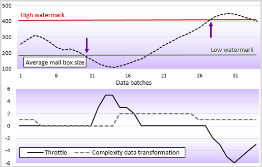
The bottom graph displays the action of the controller (throttling). The Y-axis display the intensity of the throttle from -6 for significant decrease in load (size of batches) to +6 for significant increase in load/pressure on the workers. A throttle index of 0 means that no action is taken by the controller.
The top graph displays the average size of the worker's mailbox, in response of action taken by the controller.

This implementation of a feedback controller loop is rather crude and mainly described as an introduction to the concept of back pressure control. Production quality implementation relies on:
  • TCP-back pressure using reactive streams
  • A more sophisticated throttle algorithm to avoid significant adjustment or resonance
  • Handling dead letters in case the throttle algorithm fails and the mailbox overflows

References

Saturday, November 29, 2014

Apache Spark/MLlib for K-means

Target audience: Intermediate
Estimated reading time: 5'


This post illustrates the Apache Spark MLlib library with the plain-vanilla K-means clustering (unsupervised) algorithm.


Table of contents


Overview

Apache Spark attempts to address the limitation of Hadoop in terms of performance and real-time processing by implementing in-memory iterative computing, which is critical to most discriminative machine learning algorithms. Numerous benchmark tests have been performed and published to evaluate the performance improvement of Spark relative to Hadoop. In case of iterative algorithms, the time per iteration can be reduced by a ratio of 1:10 or more.
The core element of Spark is Resilient Distributed Datasets (RDD), which is a collection of elements partitioned across the nodes of a cluster and/or CPU cores of servers. An RDD can be created from local data structures such as list, array or hash tables, from the local file system or the Hadoop distributed file system (HDFS).

Note: The code presented in this post uses Apache Spark version 1.3.1. There is no guarantee that the implementation of the K-means in this post will be compatible with future version of Apache Spark.

Apache Spark RDDs

The operations on an RDD in Spark are very similar to the Scala higher order methods. These operations are performed concurrently over each partition. Operations on RDD can be classified as:
* Transformation: convert, manipulate and filter the elements of an RDD on each partition
* Action: aggregate, collect or reduce the elements of the RDD from all partitions

An RDD can persist, be serialized and cached for future computation. Spark provides a large array of pre-built transforms and actions which go well beyond the basic map-reduce paradigm. Those methods on RDDs are a natural extension of the Scala collections making code migration seamless for Scala developers.

Apache Spark supports fault-tolerant operations by allowing RDDs to persist both in memory and in the file systems. Persistency enables automatic recovery from node failures. The resiliency of Spark relies on the supervisory strategy of the underlying Akka actors, the persistency of their mailboxes and replication schemes of HDFS.
Spark is initialized through its context. For instance, a local Spark deployment on 8 cores, with 2 Gbytes allocated for data processing (RDDs) in memory only storage level and 512 Mbytes for the master process is defined by creating a spark configuration instance of type SparkConf

import org.apache.spark.{SparkConf, SparkContext}
import org.apache.spark.storage.StorageLevel
 
val sparkConf = new SparkConf()
            .setMaster("local[8]")
            .setAppName("SparkKMeans")
            .set("spark.executor.memory", "2048m")
            .set("spark.storageLevel", "MEMORY_ONLY")
            .set("spark.driver.memory", "512M")
            .set("spark.default.parallelism", "16")
 
implicit val sc = new SparkContext(sparkConf))


Apache Spark MLlib

MLlib is a scalable machine learning library built on top of Spark. As of version 1.0, the library is a work in progress. The main components of the library are:
  • Classification algorithms, including logistic regression, Naïve Bayes and support vector machines
  • Clustering limited to K-means in version 1.0
  • L1 & L1 Regularization
  • Optimization techniques such as gradient descent, logistic gradient and stochastic gradient descent and L-BFGS
  • Linear algebra such as Singular Value Decomposition
  • Data generator for K-means, logistic regression and support vector machines.
The machine learning byte code is conveniently included in the spark assembly jar file built with the simple build tool, sbt.
Let's consider the K-means clustering components bundled with Apache Spark MLlib. The K-means configuration parameters are:
  • K Number of clusters (line 4)
  • maxNumIters Maximum number of iterations for the minimizing the reconstruction error< (line 5)/li>
  • numRuns Number of runs or episode used for training the clusters (line 6)
  • caching Specify whether the resulting RDD has to be cached in memory (line 7)
  • xt The array of data points (type Array[Double]) (line 8)
  • sc Implicit Spark context
 1
 2
 3
 4
 5
 6
 7
 8
 9
10
11
12
13
14
15
16
17
18
19
20
21
22
23
import org.apache.spark.mllib.clustering.{KMeans, KMeansModel}
 
class SparkKMeans(
    K: Int, 
    maxNumIters: Int, 
    numRuns: Int,
    caching: Boolean,
    xt: Array[Array[Double]]) (implicit sc: SparkContext) {
   
 
  def train: Try[KMeansModel] = {
    val kmeans = new KMeans
    kmeans.setK(K)
    kmeans.setMaxIterations(maxNumIters)
    kmeans.setRuns(numRuns)
   
    val rdd = sc.parallelize(xt.map(new DenseVector(_)))
    rdd.persist(StorageLevel.MEMORY_ONLY)
    if( caching )
       rdd.cache
    kmeans.run(rdd)
  }
}

The clustering model is created by the train method (line 11). Once the Spark/MLlib K-means is instantiated and initialized (lined 12 -15), the ipnt data set xt is converted into a DenseVector then converted into a RDD (line 17). Finally the input RDD is fed to the Kmeans (kmeans.run)

Thursday, October 30, 2014

Scala High Order Methods: Collect & Partition

Target audience: Beginner
Estimated reading time: 4'

This post describes the use cases and typical implementation of the Scala collect and partition higher order methods.


Table of contents
Follow me on LinkedIn

The Scala higher order methods collect, collectFirst and partition are not commonly used, even though these collection methods provide developers with a higher degree of flexibility than any combination of map, find and filter.

TraversableLike.collectFirst

The method create a new collection by applying a partial function to all elements of this traversable collection, such as arrays, list or map on which the function is defined. It signature is
    def collect[B](pf: PartialFunction[A, B]): Traversable[B]

The use case is to validate K set (or samples) of data from a dataset. Once validated, these K sets are used in K-fold validation of a model generated through training of an machine learning algorithm: K-1 sets are used for training and the last set is used for validation. The validation consists of extracting K samples arrays from a generic array then test that each of these samples are not too noisy (standard deviation does not exceed a high threshold.

. The first step is to create the two generic functions of the validation: breaking the dataset into K sets, then compute the standard deviation of each set. This feat is accomplished by the ValidateSample trait

 1
 2
 3
 4
 5
 6
 7
 8
 9
10
11
12
13
14
15
16
17
18
19
val sqr = (x : Double) => x*x

trait ValidateSample {
  type DVector = Array[Double]

    // Split a vector into sub vectors
  def split(xt: DVector, nSegments: Int): Iterator[DVector] =  
    xt.grouped(((xt.size/nSegments).ceil).toInt)
 
  lazy val stdDev = (xt: DVector) => {
    val mu = xt.sum/xt.size
    val var =(xt.map(_ - mu)
              .map(sqr(_))
              .reduce( _ + _))/(xt.size-1)
    Math.sqrt(var)
  }
 
  def isValid(x: DVector, nSegments: Int): Boolean
}

The first method, split breaks down the initial array x into an indexed sequence of segments or sub-arrays. The standard deviation stdDev is computed by folding the sum of values and sum of squared values. The value is defined as lazy so it is computed on demand once for all. The first validation class ValidateSampleMap uses a sequence of map and find to test that all the data segments extracted from the dataset have a standard deviation less than 0.8

class ValidateWithMap extends ValidateSample {
   override def isValid(x: DVector, nSegs: Int): Boolean =
       split(x, nSegs).map( stdDev(_) ).find( _ > 0.8) == None
}

The second implementation of the validation ValidateSampleCollect uses the higher order function collectFirst to test that all the data segments (validation folds) are not very noisy. collectFirst requires a PartialFunction to be defined with a condition of the standard deviation.

class ValidateWithCollect extends ValidateSample {
   override def isValid(x: DVector, nSegs: Int): Boolean =
     split(x, nSegs).collectFirst { 
        case xt: DVector => (stdDev(xt) > 0.8) } == None
    }
}

There are two main differences between the first implementation combining map and find and collectFirst implementation
  • The second version requires a single higher order function, collectFirst , while the first version uses map and find.
  • The second version throws a MatchErr exception as soon as a data segment does not comply
These two implementations can be evaluated using a simple driver application that takes a ValidateSample as argument.

 1
 2
 3
 4
 5
 6
 7
 8
 9
10
11
12
13
14
15
16
val rValues = Array.fill(NUM_VALUES)(Random.nextDouble)
  
Try ( 
  new ValidateWithMap(0.8).isValid(rValues, 2) 
).getOrElse( false)
 

Try ( 
    new ValidateWithCollect(0.8).isValid(rValues, 2) 
) match {
    case Success(seq) => {}
    case Failure(e) => e match {
    case ex: MatchError => {}
    case _ => {}
  }
}


TraversableLike.collect

The method collect behavior similar to collectFirst. As collectFirst is a "partial function" version of "find", then collect is the "partial function" version of "filter".

def filter1(x: DVector, nSegments: Int): Iterator[DVector] = 
  split(x, nSegments).collect(pf)
  
def filter2(x: DVector, nSegments: Int): Iterator[DVector] = 
  split(x, nSegments).filter( stdDev( _ ) > ratio)


TraversableLike.partition

The Higher order method partition is used to partition or segment a mutable indexed sequence of object into a two indexed sequences given a boolean condition (or predicate).
def partition(p: (A) ⇒ Boolean): (Repr, Repr)
The test case consists of segmenting an array of random values, along the mean value 0.5 then compare the size of the two data segments. The data segments, segs should have similar size.

final val NUM_VALUES = 10000
val rValues = Array.fill(NUM_VALUES)(Random.nextDouble)
 
val segs = rValues.partition( _ >= 0.5)
val ratio = segs._1.size.toDouble/segs._2.size
println(s"Relative size of segments $ratio")

The test is executed with different size of arrays.:
NUM_VALUES  ratio
     50       0.9371
 1000       1.0041
10000      1.0002
As expected the difference between the two data segments size converges toward zero as the size of the original data set increases (law of large numbers).